There could be a wide range of different reasons why generating random numbers could be useful in Excel. In this article, we will go through how to generate a random number in Excel, how to select a random value from a list or table and how to generate a random table of numbers.
Generating a Random Number
Random Number Within a Range
To generate a random number, we can use the RANDBETWEEN function. With this function, we need to enter two variables – min and max. This sets the range which the random number must lie in between.
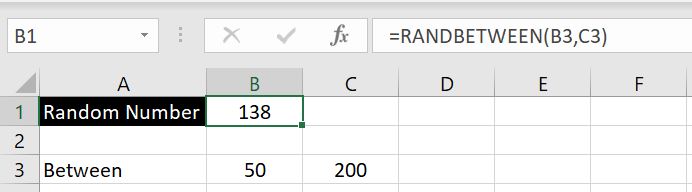
Note that if we try to set a min that is a larger number than the max, we will get the #NUM error. But they can the same number. And if the min or max are not numbers, the RANDBETWEEN function will return with #VALUE. We can enter a decimal number for min and max but RANDBETWEEN will return a whole number (integer). Negative numbers work for min and max as well.
Random Number In Multiples
When we create random numbers, we often need to set parameters and limitations around what the numbers could be. In the section above, we know that RANDBETWEEN function allows us to set a range between which the number could lie. But we could also set additional parameters such generating numbers that are in multiples of 5s or 10s or 100s or the number must be an even number.
We will do this by combining RANDBETWEEN function with the MROUND function. We have used the RANDBETWEEN function above. MROUND is an Excel built-in function that rounds a number to a specific multiple we specify. With this function, there are two variables we need to enter: 1) the number that requires rounding and 2) the multiple to which the number in 1) should round to. As a quick example:
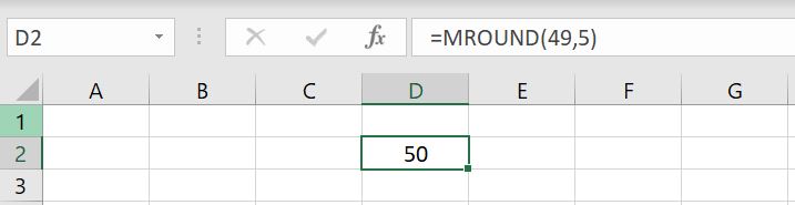
In this case, we’ve entered the number 49 and we want to round it to nearest multiples of 5. And the MROUND function returns the value of 50.
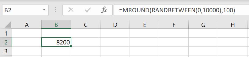
Combining RANDBETWEEN and MROUND functions, we can first generate a random number within a specified range and then have the number rounded to a multiple we specify. In the example below, we will generate a number between 0 to 10000 and round it to multiples of 100:
There is one thing to be careful with this:
- It is possible for MROUND to round the random number to a number that is outside the range we specify in RANDBETWEEN
As an example:
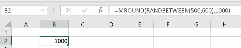
In this instance, we’ve set a range of 500 to 600 for RANDBETWEEN but because we are using MROUND to round the result to nearest thousand, Excel has returned a result of 1000. Conversely if we set the range to be 0 to 499 and MROUND with 1000 multiple, Excel will always guarantee to return the result of 0.
Random Decimal Between 0 and 1
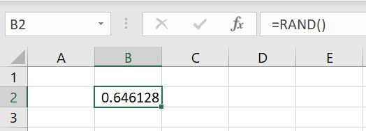
There’s a built-in function in Excel which allows users to a random decimal number between 0 to 1. It is the RAND function. This function requires no variable input. To use this function, simply enter “=RAND()”:
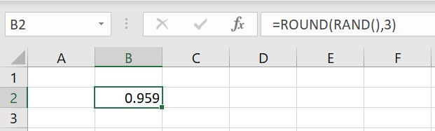
We could then use the ROUND function to specify how many decimal places we want from this RAND function. For example we could specify to only want 3 decimal places for this number:
Generating a Table of Random Numbers
To generate an array of random numbers, there is an Excel built-in function called RANDARRAY. There are 5 variables that could be entered.
- Row
- Column
- Min
- Max
- Integer/Decimal
They’re all optional as you can tell with the square brackets. And by default if we just enter “=RANDARRAY()”, Excel will generate one number between 0 to 1 and it will be a decimal. This means by default, without entering any variables RANDARRAY and RAND are very much the same. But of course by giving us the option to enter the 5 fields, we can do a lot more with this function.
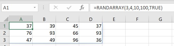
In the example below, we will create a 3 by 4 table of random numbers between 10 to 100 and they’re all integers:
Generating a Random Number (Bigger Than One)…With Decimals
So far we’ve gone through the RAND function, the RANDBETWEEN function and the RANDARRAY function. The limitation between RAND and RANDBETWEEN is that RAND only generates a number between 0 to 1 and RANDBETWEEN only generates whole numbers (integers). What if we want to generate a decimal number but larger than one?
We can use the RANDARRAY function. But instead of creating an array or a table, we will set the function to generate a 1 row by 1 column array:
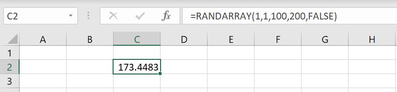
In this case, we’ve set row and column to 1 which means only one number will be generated. We’ve then set the range (min and max) for which the number to be generated. Lastly, we specified that we want the number generated to be a decimal number.
And of course similar to sections above, we could combine this with the ROUND function to specify how many decimal places we want. Or if generating integers, we could use MROUND function to round the number to the nearest multiple of our choice.
Selecting a Random Text from a List/Table
In the Index and Match – A More Advanced Lookup article, we went through how to use the INDEX and MATCH functions to look up a value. In summary, an INDEX function allows us to search for an item or a value in an array of data, given a specific row number and a column number. Given the section above, we can generate a random number with the RANDBETWEEN function and also set a range as to where the number needs to lie in between. This means we can use RANDBETWEEN to generate a random row number and/or column number in the INDEX function.
In this case we have a list of names in Column A:
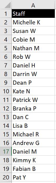
To use INDEX function to return “Daniel M”, we could do “=INDEX(A1:A20, 17, 1)”. This is because “Daniel M” is row 17 in the A1:A20 range and in Column A – first column. But suppose we don’t want “Daniel M” to be returned and we want to have a random person, we can replace “17” with a RANDBETWEEN function:
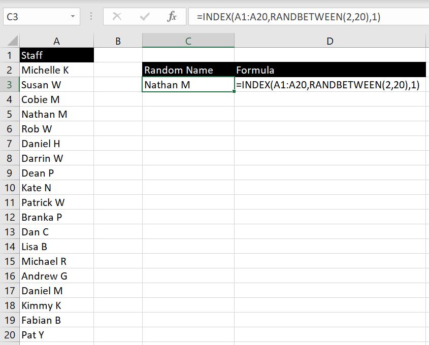
=INDEX(A1:A20, RANDBETWEEN(2,20), 1)
In this case, we are using RANDBETWEEN function to generate a random number between 2 to 20. The reason why 1 is not the minimum is because Cell A1 is “Staff” and that is only a heading so we don’t want that returned from the INDEX function.
This also works when data is not in a single column but in a table. In the example above, we’ve set the column number to 1. But we can set another RANDBETWEEN for the column number. We just need to be careful with setting the min and max for each. In the example below, the table goes from row 2 to 7 hence the function is RANDBETWEEN(2, 7). And it goes across three columns hence column number is RANDBETWEEN(1, 3).
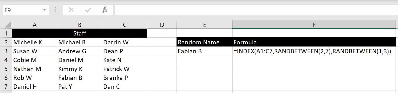
And this is how we can select a cell randomly from a list or from a table.
In this article we have gone through how to generate random numbers and set parameters on the numbers. This includes requiring the numbers to fall within a particular range and rounding the random number to its nearest multiples. We also went through how to generate a table/list of random numbers and also how to randomly select a value from a list or a table. If there is anything else you would like us to include in this article, please leave a comment below!
0 Comments Leave a comment