There are many different ways to compare two columns. And it depends on how we want to do the comparison? Do we want to simply see if item in one column is in the second column? Do we want to count how many rows have different items? Do we want to specify which rows have the same items and which don’t? In this article, we will go through as many as of these scenarios possible.
Comparing Line By Line

When we have two columns of data, one way to compare the two columns could be to simply see if the names/items for each row match. In this case, we can do so with an IF function:

=IF(A2=B2,”Y”,”N”)
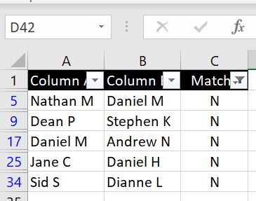
And then to highlight the rows that do not match, we can apply filter (CTRL & Shift & L):

In the example below we will look at how we can specify what the difference is.
Specifying What The Difference Is
What if instead of simply stating each row matches or not, we want to specify what the difference is? We can do that with a slight variation to the IF function:

=IF(A2=B2,”Match”,“Column A -“&A2&” and Column B -“&B2)
All we have really changed here in the IF function is what the function should return should Column A not match Column B. And instead of simply returning “N”, we have a bunch of strings that are concatenated together by “&”.
We can easily edit the formula to have it return different values in various different formats. If you have any particular format you would like to see and you are stuck, feel free to leave a comment below!
Total Number of Lines That Are Different
Now what if we don’t care which rows match and which ones don’t and we only want to know the total number of rows that match and the total number of rows that don’t? Well here it is:

=SUM(IF(A2:A34=B2:B34,1,0))
=SUM(IF(A2:A34<>B2:B34,1,0))
To break the first formula down, what we have is:
- If A2 equals B2 then Excel will return 1. If they are not the same, then return 0. By putting the entire arrays in the formula (A2:A34 and B2:B34), we can have Excel compare A2 with B2, A3 with B3, A4 with B4 and so on… And by nesting the whole formula within a SUM function, Excel adds all the 1s and 0s together.
The second formula is very similar except this time we are changing the logical test in the IF function. This time we don’t want the two columns to equal (=) each other but we want 1 to return when they are different (<>).
What is in First Column but not in Second Column?
In the section above, we were comparing the two columns row by row. But what if we simply want to see if names/items in the first column is or is not in the second column? So in this case, the order of the list does not matter.

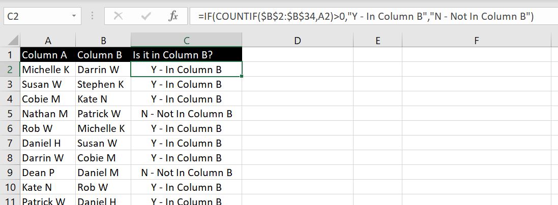
=IF(COUNTIF($B$2:$B$34,A2)>0,”Y – In Column B”,”N – Not In Column B”)
We’ve put the list in Column B in a random order. To break the formula down, we are using COUNTIF function to see if each name/item in Column A is in Column B. As long as Excel returns a result that is more than 0, it will return “Y – in Column B” otherwise it will return “N – Not in Column B”.
Once again we can use filter to see which items are not in Column B:

How Many In First Column Can Be Found in Second Column?
In this scenario we simply want to know the total number of names/items that appear and not appear in Column B:

=SUM(IF(COUNTIF($B$2:$B$34,A2:A34)>0,1,0))
=SUM(IF(COUNTIF($B$2:$B$34,A2:A34)=0,1,0))
Breaking the first formula down, we are using COUNTIF to see if A2 is in Column B. If the result is more than 0, then Excel will return 1 otherwise it will return 0. By putting the criteria as an array A2:A34, we are getting Excel to run this COUNTIF from A2 down to A34. Without the SUM function, Excel will list down all the results (1 or 0). By nesting this into a SUM function, Excel will add all results (1s and 0s) together and return the total.
The second formula is very similar, except we want COUNTIF to return 0. This will indicate to us the name/item in Column A is not in Column B. The best way to check our work is that the total of these two results (21 and 12) add up to the total number of names/items in Column A.
Have we missed anything? How would you like to compare two columns? Leave us a comment to let us know what you need and we will add it onto this article!

0 Comments Leave a comment