Pivot Tables in Excel are useful when it comes to summarizing and analyzing a large amount of data. They are often used because they are easy to set up and edit. Pivot tables can help us look at large dataset in various different angles. The end result is easy to read and understand hence it is often used for reporting and presentation purposes. When data is updated, Pivot Tables can be updated by simply clicking “Refresh”. Because of that, Pivot Tables are very useful when used with Power Query which is a great tool in automating and simplifying regular reportings. Click here to see what Power Query is and how it works.

• How To Create Pivot Tables
• Setting up Pivot Tables
  • Filters
  • Rows & Columns
  • Values
• Refreshing the data
• Different Layouts
• GETPIVOTDATA function (instead of VLOOKUP)

How To Create Pivot Tables

The steps to creating pivot tables are simple.

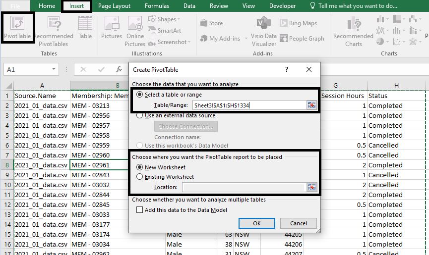
1. Click on any cell in the table of data
2. Go to Insert tab and click on PivotTable
3. Choose where we want the PivotTable – usually select New Worksheet. However if we have an existing worksheet in the file where we want to create the PivotTables, we can also select Existing Worksheet. (Before clicking Ok, have a quick look to make sure the data range selected is correct)
4. Click Ok

Setting up Pivot Tables in Excel

Creating Pivot Tables is the easy bit. Knowing how to create the Pivot Tables we want and navigate through all the different settings is often the tricky and confusing part.

In the PivotTable Fields, there are 4 fields: Filters, Columns, Rows, Values. We will first go through each one:

Filters

We can drag different fields into the Filters section. And yes we can drag more than one fields into this section. Once a field is in the Filters area, it appears at the top of the table. We will then be able to use filter to select the information we want to see for this particular table. For example, we can filter Status to only look at sessions with “Cancelled” status.

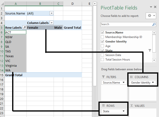
Rows & Columns

Rows & Columns sections are much more straight forward. Have a look at image below to see how it works. Note: you don’t have to have both rows and columns. It is perfectly fine to have one or the other.

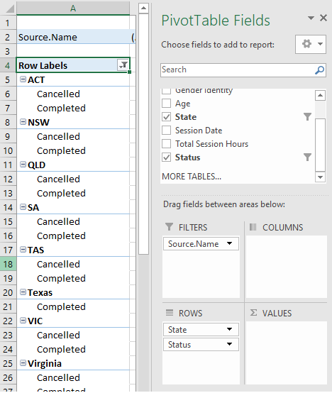
For slightly more advanced Pivot Tables, we can also have multiple fields in Rows and/or Columns. Note: the order in which we place the fields in the Rows section is important. For example if we put State on top of Status, we get different statuses within each state (shown in image below on the left). But if we have Status on top of State, then we will have different states within each status (shown in image below on the right):

Values

The Values area allows us to select what we want to count or calculate for this table. For non-numerical fields, it will simply do a count. Using the example below, we are counting how many members there are in each state:

For numerical fields, we have more options. For example, if we change the field in VALUES section from Member No. to Total Session Hours, we will have the option to do other calculations. We can click on the field and select Value Field Settings:

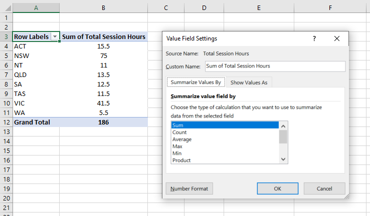
We can count the number of sessions or we can calculate the total number of hours. Alternative we can also do other calculations such as find the maximum/minimum/average, multiplication and standard deviation…

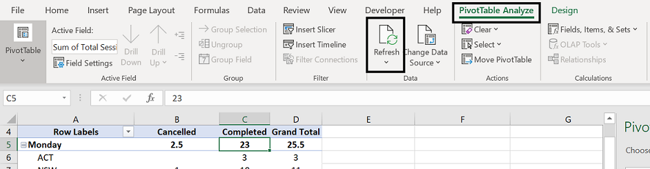
Refreshing the Table

Refreshing data in Pivot Tables is very simple. We can do that by simply following these three steps:

1. Click on anywhere in the Pivot Table
2. Go to PivotTable Analyze at the top
3. Click on Refresh

Different Layouts to the Pivot Table

There is a few different ways to format Pivot Tables.

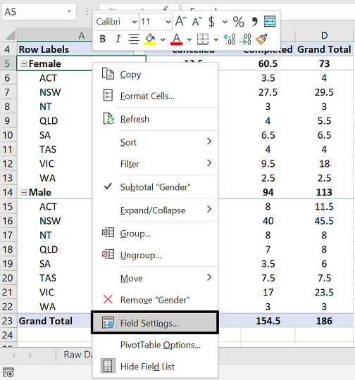
1) Right-click on the heading and select Field Settings:

2) Go to the the Layout & Print tab. Play around with different options here. As an example here, we will select:

• “Show item labels in tabular form”
• “Repeat item labels”

And this will be the new layout:

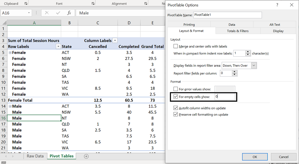
There are also other layouts options. We can right-click, select PivotTable Options. There we can make more changes to layout options. For example below, we can choose what we want to see for empty cells:

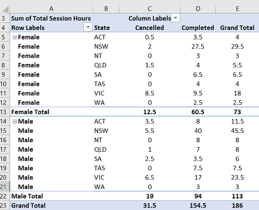
And the table will look a lot neater. And the best thing about Pivot Tables is we only have to change the settings and set the layout once:

GETPIVOTDATA Function

Because PivotTables are so flexible, the table can be adjusted all the time depending on the data and the settings. VLOOKUP function may not be the best function to use because the number of columns changes. But Excel has a GETPIVOTDATA function.

=GETPIVOTDATA(data_field, pivot_table, [field 1, item 1], [field 2, item 2]…)

Getting Table Grand Total

With the GETPIVOTDATA function, only the first two inputs are mandatory fields:

• data_field: name of the table which can be located at the top left of the table
• pivot_table: cell reference to that table name

If we only enter the first two fields, the function returns the grand total of the whole table:

With this function, it doesn’t matter how data in the Pivot Table changes, the GETPIVOTDATA function will always return the grand total.

Getting Row/Column Total

As we add more and more information into the GETPIVOTDATA function, we can be more specific in terms of which row/column we want to gather data in:

=GETPIVOTDATA(data_field, pivot_table, [field 1, item 1])

• data_field: name of the table which can be located at the top left of the table
• pivot_table: cell reference to that table name
• field 1: name of the row/column field
• item 1: specific row/column we are looking for

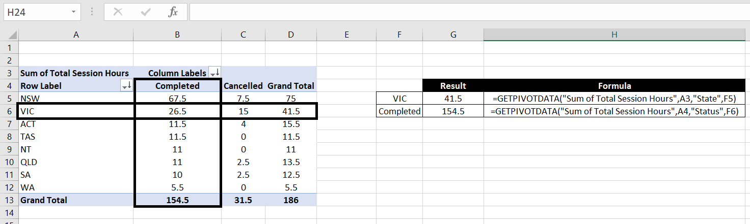
Note: it is important to get the name of the row/column correct. It’s the name of the field, not “Row Label” or “Column Labels”. If you can’t remember, you can right-click on the Pivot Table, select Show Field List and check: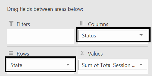 Also, Grand Total is not considered a field in row/column. This means =GETPIVOTDATA(“Sum of Total Session Hours”,A3,”State”,“Grand Total”) will not work. To get the grand total of the Pivot Table, refer to section above on Get Row/Column Label.

Getting Specific Data by Row & by Column

Not a surprise here, following on from above, we will add more information into the GETPIVOTDATA function so we can get data for a specific row and column:

=GETPIVOTDATA(data_field, pivot_table, [field 1, item 1], [field 2, item2]…)

• data_field: name of the table which can be located at the top left of the table
• pivot_table: cell reference to that table name
• field 1: name of the row/column field
• item 1: specific row/column we are looking for in field 1
• field 2: name of the second row/column field
• item 2: specific row/column we are looking for in field 2
• and so on…

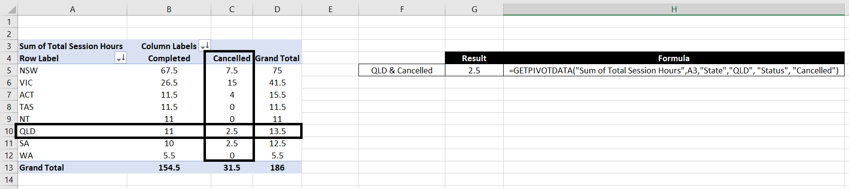
As mentioned in section above, be careful with getting the name of the row and column correct. They are names of the fields, not “Row Labels” or “Column Labels”. And following the same logic, we can use this formula for tables that have multiple rows.