How can we look for a partial value with VLOOKUP? We know that VLOOKUP function has the option to not look for exact match but the list would have to be sorted in order first. And even then it is not very accurate. In this article we will first look at how to do a VLOOKUP when we only know part of the lookup value. And then we will look at how VLOOKUP with “approximate match” actually works and why it does not always return the expected results.

Partial Value with VLOOKUP

VLOOKUP function in Excel allows for lookup of a partial value. Imagine having information below and you can’t quite remember the last name of an employee but you definitely remember his first name is “Dean”:

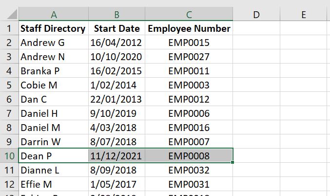
With VLOOKUP function, we could use search for partial values by adding the asterisk * to the lookup value. Here’s an example:

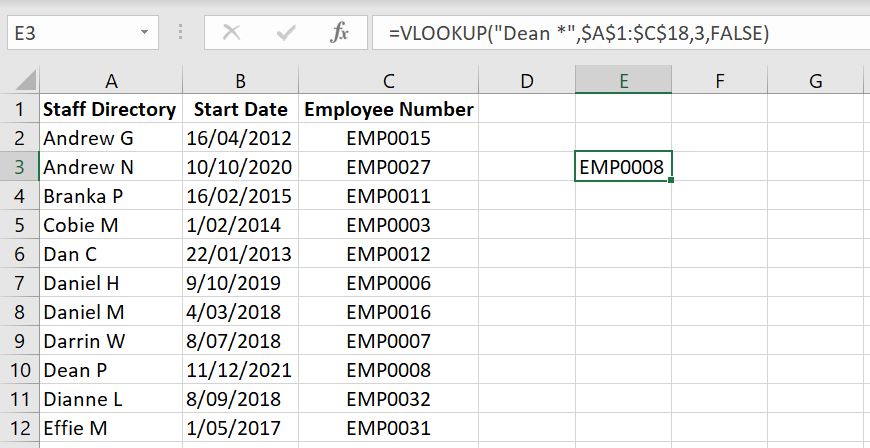
=VLOOKUP(“Dean *”, $A:1:$C:$18, 3, FALSE)

And we are not restricted to adding this to the end of the value. We could also add the asterisk to the beginning of the lookup value. Here’s another example:

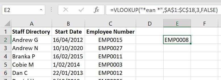
=VLOOKUP(“*ean*”, $A$1:$C:$18, 3, FALSE)

Cell Reference with Partial Value

In both examples above, we used VLOOKUP by typing in the lookup value into the function and adding asterisk(s) to it. But what if we want to reference another cell and add an asterisk to the lookup value?

=VLOOKUP(E2&”*”,$A$1:$C$18,3,FALSE)

And once again we can also add the asterisks to the beginning of the lookup value:

=VLOOKUP(“*”&E2&”*”,$A$1:$C$18,3,FALSE)

Essentially we are attaching a “*” to the lookup value and because this time it goes with a cell reference, we need to link them together with &.

VLOOKUP with APPROXIMATE MATCH

For VLOOKUP with approximate match, Excel has made it clear that the array of data needs to first be sorted in order: VLOOKUP Function

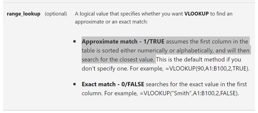
But even then, does it give us the results we are expecting? Let’s have a look. And let’s keep in mind, because we are looking at an approximate match here, there’s probably no right or wrong answer. It really is just how it works with Excel. Note that to sort the array in numerical or alphabetical order, instead of rearranging the whole table, we can make use of the SORT function. For example:

• =VLOOKUP(A2, SORT(A2:C100), 3, TRUE)

But to better illustrate how VLOOKUP with approximate match works, we will sort our data in order so it is easier to see the result and make sense of it.

Numerical Lookup Values

First we will use numerical lookup values. And to clearly demonstrate how the function works, we will list down a list of numerical values as lookup values:

In the example above, we’ve used lookup values of 100.01, 101, 101.99, 102 and 102.01.

The 100.01, 101.00 and 101.99 are lookup values there used to show VLOOKUP function with approximate match does not round up any numbers for us. In fact it will keep going down the list from the top until the lookup value is smaller than or equal to the value in the left column. It is interesting to note that although 101.99 is so much closer to 102, Excel will still see 100 as the “approximate match” and return “EMP0001” as the result.

102 is an exact match. It returned the expected result although we specified an “approximate match”, which is good. 102.01, very similar to 100.01, because it is smaller than 104 which is the next value after 102, gets rounded back down to 102 as the approximate match and so “EMP0002” is returned.

As mentioned before, there is no right or wrong answer. It is just how Excel works. It could be useful in some cases. It is just important to know exactly how it works. With this in mind, let’s explore how this function will work with non-numerical values.

Strings and Texts as Lookup Values

With text and strings as lookup values, let’s remove the File Numbers currently in Column A and sort the Staff Directory in order:

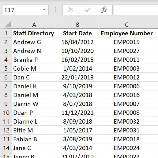
Again we will use a list of different lookup values to demonstrate how the VLOOKUP works with “approximate match” for non-numerical values:

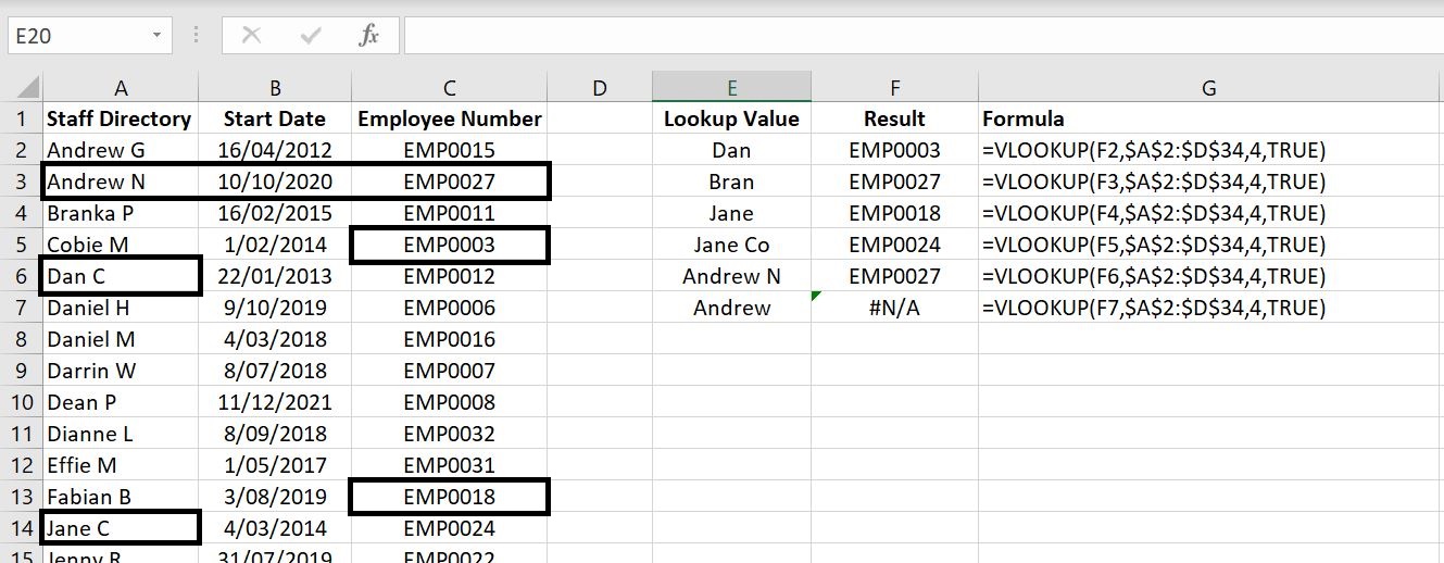
Let’s first look at the lookup values with “Dan”, “Bran” and “Jane”. This is actually very similar to the results in the numerical section above. Each function is returning the result of the row above. “Dan” is not quite the same as “Dan C” so it returns the line above and hence we have EMP0003. Similar with “Bran” and “Jane”.

However with lookup value of “Jane Co”, because this actually meets the criteria of “Jane C” and has more characters to it, Excel returns the correct employee number: “EMP0024”. Alternatively maybe the better way to look at it is:

• In the table, the line under “Jane C” is “Jenny B”. But because “Jenny B” is clearly after “Jane C” alphabetically, Excel returns the previous line as the “approximate match”. So we can basically approach how VLOOKUP with “approximate match” works based on how we would search for words in a dictionary. As soon as we’ve gone past that word alphabetically, the one immediately before that will be the “approximate match”.

Once again with exact match “Andrew N”, Excel returns the expected result. In this case, it is EMP0027.

Following very similar logic as above, with “Andrew”, because it is the top result, there is no row above that which Excel would look for – remember the array used here starts with A2. Hence it cannot go into Row 1 and that is why Excel is returning with a #NA error.

In this article, we went through how to use VLOOKUP function with partial look up values and also how VLOOKUP function works with “approximate match”. If there is anything you wish us to add onto this article, leave a comment below! We look forward to keep improving our articles.