The VLOOKUP function searches for the lookup_value in the leftmost column in the table_array and stops when the first match is found. But what if there are multiple entries in the table?

Have a look at an example below:

There are multiple “Kate N”s in the company. Using VLOOKUP, you will only get Start Date or Employee Number for the first “Kate N” in the list. So how can we get the full list of Start Dates or Employee Numbers for all “Kate N”s.

FILTER Function in Excel

The FILTER Function is perfect for the occasion and is simple to use.

The FILTER function is:

• =FILTER(array, include, [if_empty])
• 
  array: the range of cells you want returned
• include: the value to search for and the range of cells to look for that value
• [if_empty]: what should the function return if nothing can be found

In order words, with the FILTER function, we first enter the range of cells which we want Excel to possibly return. And then we specify what the lookup value is and the range of cells Excel should look for that value. In the example below:

• array: Employee Numbers which is the C2:C34 range
• include: the value to search for which is “Kate N” in E2 and we want Excel to look for that in the Staff Directory list which is the A2:A34 range

In the example above, we did not use [if_empty]. It is an optional field. It specifies what should be returned if the lookup value cannot be found. For example below, we can specify “Not Found” to be returned if staff’s name in E2 is not in the Staff Directory list in column A.

If you choose to not use the [if_empty] field, you will get a #CALC error when the lookup value cannot be found.

Right to Left (Unlike VLOOKUP)

Another advantage the FILTER function has over VLOOKUP is that VLOOKUP must start searching for the lookup value in the leftmost column and can only return a value on the right side of that value in that row. With FILTER function, you can move start from the right and look for a value in the right side column and have Excel return a value on the left:

This means we could specify an Employee Number and find the name of the staff without having to rearrange the columns in the table. This would not be possible with VLOOKUP.

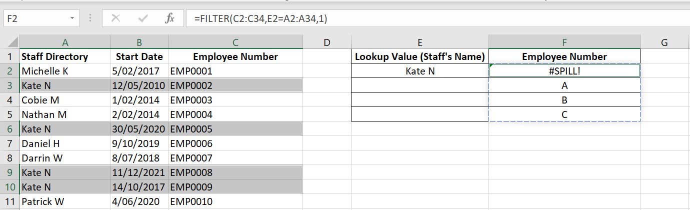
#SPILL Error in FILTER function

#SPILL error appears with FILTER function when Excel wants to return multiple results but the cells below are not empty. In the example below, there are four “Kate N”s and hence there are four Employee Numbers the FILTER Function would like to return. But F3:F5 already have data in those cells (“A”, “B” and “C”). Once “A”, “B” and “C” are removed, #SPILL will disappear.

We hope you find this article useful. If you have any more questions on this topic, please leave a comment below and we will keep editing this article to make it more and more useful for everyone.