Similar to the COUNTIF function, SUMIF is also one of the most fundamental functions to use in Excel when it comes to reporting and data analysis. In this article, we will go through how this function works and also explain why values may not be adding up correctly. We will also apply multiple conditions in SUMIFS function. And we will set conditions with greater than/less than or equal to.

SUMIF – How It Works

Let’s first go through the basics of how the SUMIF function works. And as obvious as it sounds, we should start by explaining what the function does. SUMIF is a:

• Built-in Excel function that allows users to calculate the sum of certain values if a condition is met. For SUMIF, there are three inputs/variables requires for the function: range, criteria, and [sum_range]:
  • Simply put, Excel would add up values in the array (sum_range) if values in the range meets the criteria

=SUMIF(range, criteria, [sum_range])

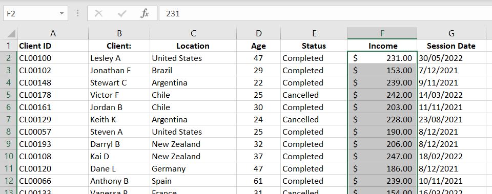
Let’s use data below as an example:

With SUMIF function, we could do more insightful analysis such as getting total income based on location or total income for each year. We could basically separate data into groups. For example we could look at total income by age brackets of the clients.

=SUMIF($C1:$C196,I2,$F1:$F196)

In this example, we are adding income (sum_range – Column F) together if the location (range – Column C) matches our criteria (I2). In Cell I2, we have “United States”. Hence for every row where we have “United States” in Column C, Excel will add the income in Column F because the condition is met. And similarly for Brazil, Argentina and other locations.

The good thing about SUMIF function is that it is not limited to the range column being on the left of the sum_range column. In the example above, we could easily have swapped Column C and Column F and SUMIF could still perform the exact same calculation for us.

Numbers Not Adding Up Correctly? Important!

Are values not adding up correctly? This, for obvious reason, is worse than getting an error. Why? Because it is not always obvious that we’ve made a mistake! This is why it is important to make sure we enter values into SUMIF function correctly, otherwise we could be getting an incorrect answer without even knowing it.

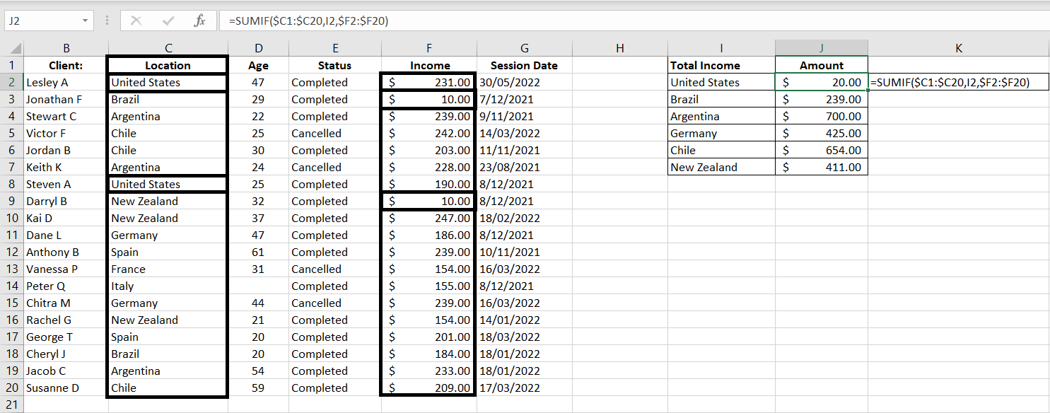
With the SUMIF function, there are two arrays we need to enter: 1) range and 2) sum_range. It is very important that the two are aligned. Especially because of headings, it is easy to make a mistake and start one array in row one and the other in row 2. To clearly illustrate the problem and how the function works, we have changed the numbers and made the table smaller to make this more obvious:

=SUMIF($C1:$C20,I2,$F2:$F20)

Notice that the range starts with Row 1 (C1) and sum_range starts with Row 2 (F2). Because of that, the corresponding rows do not match up anymore. From Excel’s perspective, the second and eighth rows in range C1:C20 are “United States”, hence it will return the second and eighth rows in sum_range F2:F20. But the second and eighth rows in F2:F20 are $10 and $10. Hence the SUMIF function returns $20 as the result.

SUMIF with Dates and with Greater or Less Than

So far we have only looked at examples where the criteria and values in range are exact matches. What if we don’t want an exact match? What if we want greater than (>) or less than (<)? Or what if we want to add up values across a certain period of time?

Greater Than or Less Than…

Let’s first look at how greater than and less than work in SUMIF functions. In this simple example, we will add up values in Income column if values in Age column is 1) over or equal 35 and 2) under 35:

=SUMIF($D$2:$D$196,“>=”&35,$F$2:$F$196)

=SUMIF($D$2:$D$196,“<“&35,$F$2:$F$196)

Both are almost exactly the same except for the criteria. After all, both are looking at the same Age Column and the Income Column. In the first function, we want greater than or equal which is “>=”. And to connect that with 35, we just need to add a & in between.

Similarly with the second formula, we want a less than which is “<“. And we connect it with &35. In this case we don’t want a “less than or equal to” because the “equal to” would overlap with the first “Over or equal 35” formula.

Note: there are in fact some blank fields in the Age column but Excel would ignore them. To Excel, that means a blank cell is not the same as 0. With a “less than 35” condition, a blank cell is not considered meeting the condition. And in fact that would be perfect in our scenario, Column D is an Age column. A blank cell would more accurately be considered as “unknown“, not 0.

SUMIF with Dates

Using very similar logic, we can add up values if the dates fall within a particular range. Here we want to add up values in Income column if Session Date is prior to 2022:

=SUMIF($G$2:$G$196,“<“&DATE(2022,1,1),$F$2:$F$196)

The range we are comparing the criteria with is G2:G196. The criteria is that the value in this range must be less than “<“ 01/01/2022 which is represented by DATE(2022, 1, 1) and we again connect the two with &. We could simply put it in a regular date format with quotation marks, e.g. “01/01/2022”. However because different countries could use different date formats (e.g. mm/dd/yyyy or dd/mm/yyyy), it will be less confusing to just use the DATE(year, month, date) function.

Note: the good thing with SUMIF function with dates is that it knows to ignore blank cells in the range. That is if a cell is blank in G2:G196, it will NOT be considered as a condition met.

Tip: always check your work. If the SUMIF function that is greater than or equal to a date and another SUMIF function that is less than that same date do not add up to the total, then you would know that there’s probably a field missing in the session date.

SUMIFS – Multiple Conditions

What if we want to add multiple conditions into SUMIF function? Well luckily there is a SUMIFS function. It is literally just a SUMIF but with multiple conditions. The order we enter our variables changes slightly. With SUMIFS, it is:

= SUMIFS(sum_range, criteria_range1, criteria1, [critieria_range2, criteria2]…)

Notice that there is no square bracket around sum_range now. This means sum_range is now a mandatory field. The first set of range and criteria is also mandatory. But conditions 2, 3, 4…are optional.

=SUMIFS($F$2:$F$196,$C$2:$C$196,I2,$E2:$E196,J2)

=SUMIFS($F$2:$F$196,$D$2:$D$196,”>”&45,$E2:$E$196,J3)

The easiest way to visualize this is first we tell the function the range of cells which has the values we would like to add up (F2:F196). After that, we put in each set of criteria_range and the criteria:

• In the first example, for Column C (Location), we are looking for “United States” as the criteria (Cell I2) and also in Column E (Status), we are looking for “Completed” as the criteria (Cell J2)
• In the second formula, for Column D (Age), we are looking for values greater than 45 as the criteria and also in Column E (Status), we are looking for “Cancelled” as the criteria (Cell J3)

Sum_Range Can Be Optional?

Ever noticed that in the SUMIF function, sum_range is in square bracket? This would of course mean that this field is an optional input. The function can still work with or without this variable. Strange but it works.

If the sum_range is blank, Excel will add up values in range field. That is, of course only if values in range are numerical values. We will show two examples below:

1) Numerical Values

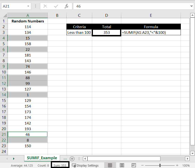
Here’s a list of random number between 0 to 200 – randomly generated by RANDBETWEEN. In this example, we will add up the numbers if they are less than 100:

=SUMIF(A1:A23,”<“&100)

We highlighted cells with values less than 100 and we can see at the bottom the “Sum: 353” matches the SUMIF result. This shows that while the criteria is being matched against the range, values in the range would be added up.

2) Non-Numerical Values

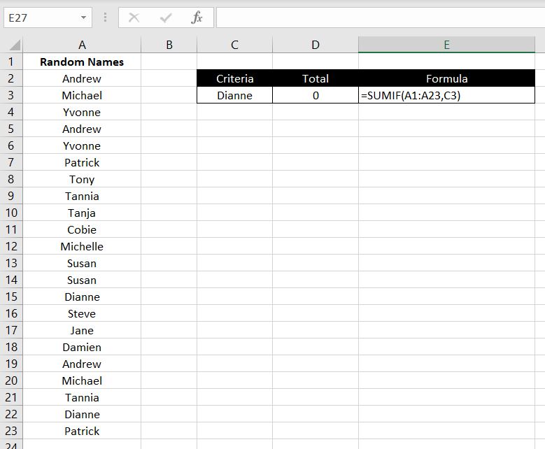
Here we are doing a SUMIF in range A1:A23 and the criteria is “Dianne”:

=SUMIF(A1:A23,C3)

Again no alert pop up appeared. Excel will happily calculate the function for us because sum_range is only an optional field. But as expected, because names are non-numerical values, there is nothing to add up. Hence the SUMIF function returns a 0.

We hope you now have a good understanding of how SUMIF works in Excel. If you need any further clarification or if you feel that we’ve missed anything, please leave a comment below.