Check boxes in Excel are a useful tool in creating checklists or to-do lists. They are simple to use. Everyone knows how to use a checklist. Users only have two options: tick the checkbox or deselect it. In this article, we will go through step by step how to add check boxes in Excel. And then more importantly we will look at how we can use the results in the checkboxes. This includes using formulas to calculate the results, setting conditional formatting based on check boxes and lastly how to add VBA/Macro into check boxes. However before we start, let’s look at the differences between check boxes and radio buttons because they are different in Excel and should be used differently.

Check Boxes vs Radio Buttons – When To Use Each One?

In the Developer tab, under the Controls Section, there is a list of Forms Controls we could insert. Two of which are check boxes and option button (radio buttons). At first glance just by looking at them, the only difference is that one is shaped as a box and the other is shaped as a button. What’s the difference and when should we use each one?

Check boxes:

• Users can select as many check boxes as they want
• Users can deselect any or all of the check boxes

Radio buttons:

• Users can only select one radio button at a time
• Selecting one button will automatically deselect all the other buttons
• Unless we go into Format Control to deselect a radio button, one button must be selected at all times within a group

Simply put, check boxes should be used if you want to be able to select multiple options. And radio buttons should be used if you only want to select one option at a time. In this article, we will only go through check boxes in Excel.

How To Add Check Boxes?

First of all, to be able to insert check boxes, we need to access the Developer tab and make sure the Excel file is saved as macro-enabled. For more instructions on that, please click here.

Once we can see the Developer tab, we can insert a check box by:

1. In the Controls section, click on Insert
2. Select Check Box:
   
   
3. Click on anywhere in the worksheet and a check box will be inserted

To generate more check boxes, we could either:

1. Copy the check box and paste as many as we want
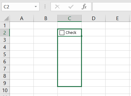
2. Align the current check box into a cell and drag the cell down or across as though we are copying a formula:
   
   
   

Formatting Check Boxes

By default, after inserting a check box, this is what the check box will look like:

In most cases, we will need to do some formatting with it. That is of course unless we just want to leave it as “Check box 1”, “Check box 2”, etc. To edit the wording next to the check box:

1. Right-click on the check box
2. Select Edit Text
   
   
3. Edit text as you wish. Note that you could have no text at all next to a check box:
   
   

To select and move the check box around:

1. Right-click on the check box to select it and then move it around, or;
2. Hold the CTRL key and click on the check box. Then we can move it around

Linking A Check Box To A Cell

Before going through how to apply formulas to check boxes or conditional formatting, we first need to know how to link a check box to a cell. By linking a check box to a cell, we can then use formulas to reference that check box by referencing the cell because they are now linked:

1. Right-click on the check box
2. Select Format Control:
   
   
3. Click on the Control tab
4. In the Cell link field, enter the cell you would like to link the check box with
   
   
5. Click Ok

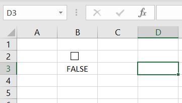
In this case, we linked the check box with Cell B3. If we now tick or deselect the check box, we can see what Excel does for us:

By selecting the check box, B3 will be updated with “TRUE”:

By deselecting the check box, B3 will be updated with “FALSE”:

As you can probably imagine, now we have a cell updating its value between TRUE and FALSE based on whether the check box is selected, we can now apply many different kinds of functions to the check box.

Before doing that, there is a couple of things to be mindful of when linking check boxes with cells:

1. Hiding TRUE/FALSE results:
   • We do not always want to see the TRUE or FALSE results. We can’t just make it disappear but we can have it not visible. First, link the check box to the cell it is actually situated in. Second, check the font color of that cell to match the cell color
2. Copying and pasting check boxes:
   • When we linked the check box to the cell (B3), it would seem like the cell reference is dynamic, meaning if we then drag the cell down to create more check boxes, they would automatically be linked to the respective cells (e.g. B4, B5, B6…). However this is not the case:
     
     
     
     Each check box is still linked to the same cell – the one that we initially linked the first one to. It does mean with each check box, we will need to manually link each one. Tip: to manually link the check box as quickly as possible:
     • Press CTRL and click on the check box to select it
     • Press CTRL & 1 to open the Format Control box

How To Calculate Results From Check Boxes Using Formulas?

Once a check box is linked to a cell, if the check box is selected, the cell will be updated with “TRUE”. And when the cell is deselected, the cell will be updated with “FALSE”. You can then imagine how we can apply different formulas with that. Here’s a practical example of how we can use check boxes to create a to-do list:

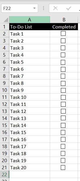
Each check box is linked to the cell it is located in.

Let’s start with something simple:

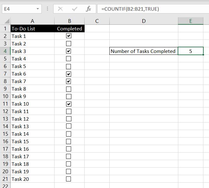
=COUNTIF(B2:B21,TRUE)

Here we are counting the number of “TRUE”s in the range B2:B21.

Next we will go through a slightly more complicated formula. To find out more about COUNT functions, please have a look at this article – All the COUNT Functions in Excel.

=IF(COUNTIF(B2:B21,TRUE)=21,“All Tasks Completed”, COUNTIF(B2:B21,”FALSE”)&” tasks outstanding”)

We will break this formula down. With this IF function, first:

1. COUNTIF(B2:B21,TRUE)=21 – we are testing if the number of “TRUE”s equal to 21
2. If the number of “TRUE”s equal to 21, the IF statement will return “All Tasks Completed”
3. Otherwise, it means there are still outstanding tasks. What happens then is we will have Excel count the number of “FALSE”s (COUNTIF(B2:B21,”FALSE”)) and concatenate that number with ” tasks outstanding”. In the example above, it is “15 tasks outstanding”.

If all the check boxes are ticked, the following will appear:

Check Boxes With Conditional Formatting

In this section, we will go through how to use conditional formatting with check boxes:

There are two sets of conditional formatting applied here:

1. Strikethrough the text in Column A if the task is completed
2. Set the cell color as red if the task is not completed

For the first condition:

1. Click on cell A2
2. Go to Home tab and in the Styles section, select Conditional Formatting > New Rule
   
   
3. In the Select a Rule Type area, select the last option: Use a formula to determine which cells to format
4. In the Format values where this formula is true field, enter “=B2=TRUE”
   
   
5. Click on Format
6. Under Effects, make sure Strikethrough is selected
   
   
7. Click Ok

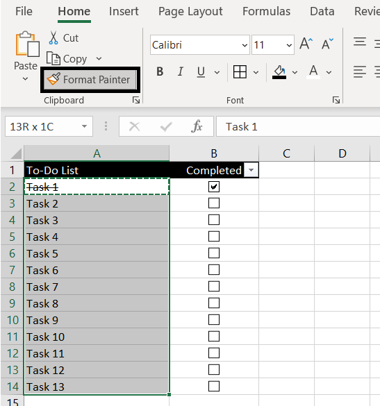
And that’s it. Conditional formatting would be done for A2. To apply this to the rest of the cells in Column A:

1. Select Cell A2
2. Click on Format Painter
3. Select the range of cells you want to apply this format to:
   
   

Tip: for this to work, make sure you didn’t use absolute referencing for B2 when setting this conditional formatting. You would need to keep it dynamic. That is, have “B2=TRUE” instead of “$B$2=TRUE”.

The second set of conditional formatting is even more straight forward. It is to set the cell color red if check box is not selected:

1. Select B2
2. Go to Home tab and in the Styles section, select Conditional Formatting > Highlight Cells Rules > Equal To
   
   
3. Here we want the cell value to equal FALSE and select Custom Format
   
   
4. In the Fill tab, select the color red
5. Because when linking the check box with the cell, we changed the font color “TRUE/FALSE” to white. Here we need to go to Font tab and make sure the color matches the color of the cell – red (or whatever color you selected in step 4)
6. Click Ok

Again, use Format Painter to copy the conditional formatting for B2 for rest of the cells.

Check Boxes With Simple VBA/Macro

When we went through the differences between check boxes and radio buttons in Excel, we mentioned that with Excel, more than one box can be selected at a time. In fact, all check boxes can be selected at the same time.

Well we can use VBA to change that. In the example below, we have two check boxes. We’ve set up and assigned VBAs to each check box such that we could have:

• Both check boxes deselected at the same time, or
• Either one of the check boxes selected at a time

But we cannot have both selected at the same time. Selecting one will automatically deselect the other. Essentially what we are doing is changing check boxes into radio buttons, except that we allow both to be unchecked, unlike radio buttons:

The VBA is very simple. What need is that every time the check box is selected, we need Excel to make sure the other check box is not also selected. And if it is, it will need to be unchecked. Note that the opposite is not true. If the check box is being deselected, no action needs to be done since in this case we want to allow for both check boxes to be unchecked. So if a check box is being deselected, it doesn’t matter if the other check box is selected or not.

1. Go to Developer tab
2. Open Visual Basic
3. Insert a Module

Follow the same step and create another module:

We now have two modules: OneOrTheOther1 and OneOrTheOther2. Because each check box is linked to its respective cell, what the VBAs are doing is if the check box is now having a “TRUE” value, the other check box must then be “FALSE”.

After creating the VBA modules, the final step is to assign the VBAs:

1. Right-click the first check box
2. Select Assign Macro
   
   
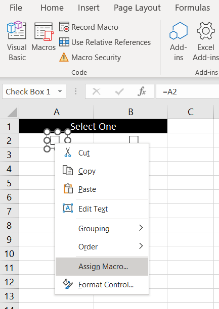
3. Select the first VBA – OneOrTheOther1
4. Click Ok

Follow the same process for the second check box and assign OneOrTheOther2.

And that’s it. Now we will only be able to select one check box at a time. And the difference between this and radio buttons of course is that we could deselect all check boxes if we wanted.

As you can imagine, by first linking the check boxes with cells, we can have “TRUE” or “FALSE” values assigned to cells. With that it’s up to our imagination what functions/formulas and VBAs we want to apply with the check boxes. If there is anything specific you would like us to go through, leave a comment below!