
3D Range is a useful tool in Excel that makes it easier for us to collate data across different tabs. This is particularly useful when we use a particular template over multiple worksheets and we want to collate everything into one sheet.
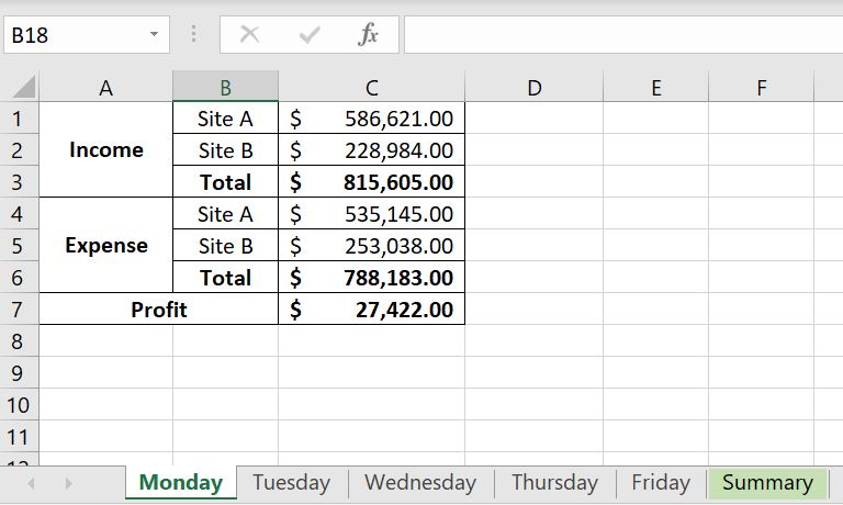
Imagine here we have a standard template to capture data across all worksheets from Monday to Friday and we want to add up the data in the “Summary” worksheet:
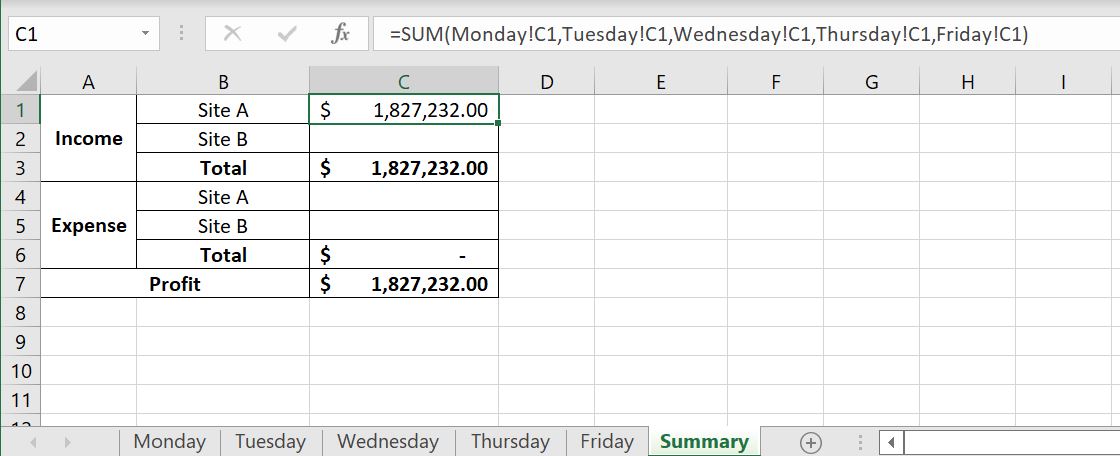
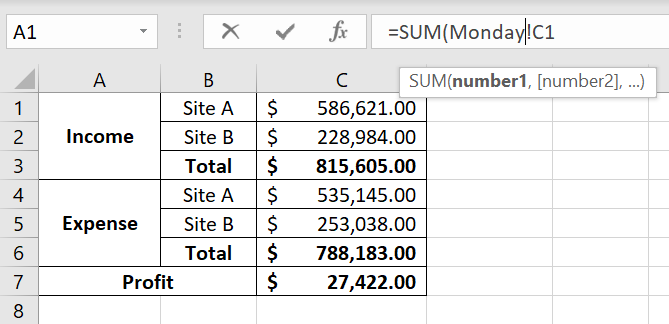
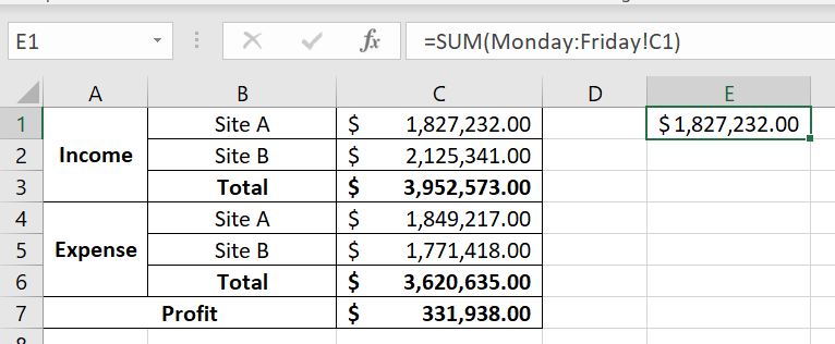
The most common way would probably be to use a SUM function, go into each worksheet and click on each cell individually. You will end up with something like this:
3D Range can make this a lot simpler. Let’s find out how.
3D Range – How Does It Work?
In Excel, when we want to refer to a range of cells, we join the first cell and the last cell with a semi-colon. For example: “A1:F40”. Well we can actually do the same with worksheets. So why is 3D range useful? It is the same logic as in situations where:
- Let’s say we want to add A1:A20 together, we would not write =SUM(A1, A2, A3, A4…A18, A19, A20). We would write =SUM(A1:A20). This is the same logic with 3D range. We can the same with worksheets.
Using the example above, we have an Excel file with “Monday” to “Friday” worksheets, each has the same template and we want to collate data into the “Summary” worksheet:
Because each worksheet has the same template, all the numbers we are adding together are all in Column C. The syntax in writing 3D Ranges is very similar to how we write a range of cells. If you want to refer to a range of cells, we would start with the first cell, put a semi-colon and then link it with the last cell. For example: A1:A20. It is very similar with 3D Range:
- Monday:Friday!
- Note that if there is a space in the name of the worksheet, we will need to put a single apostrophe around the worksheet names. For example if we add a ” 2022″ to the worksheets, the 3D Range becomes ‘Monday 2022:Friday 2022’!
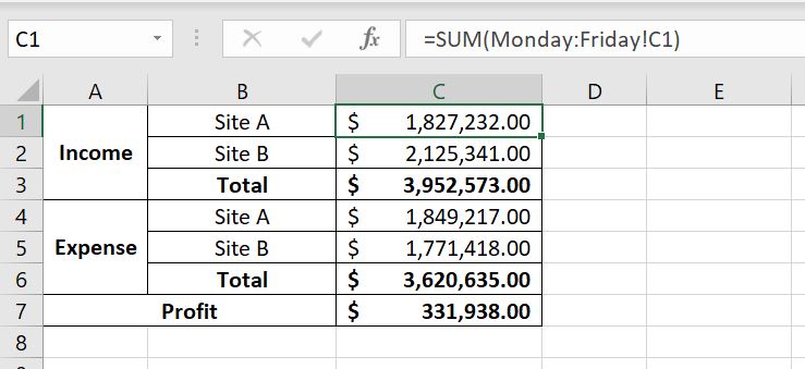
=SUM(Monday:Friday!C1)
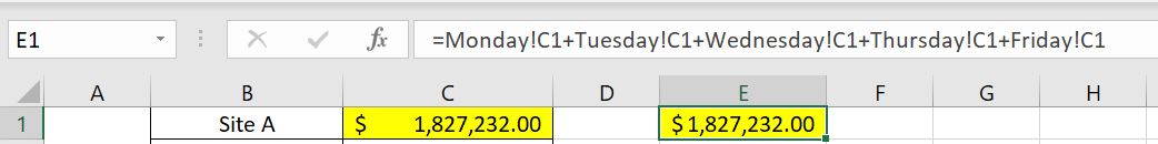
And then we can drag the formula down to fill in C2:C7. Let’s check our work by adding each cell together:
Tip On Writing 3D Ranges
Here’s a tip on how to best write 3D Ranges:
- Start with “=SUM(” in the Summary worksheet
- Click into “Monday” worksheet
- Click on the cell we would like to add:
- After “Monday”, type in “:Friday”
- Close bracket at the end of the SUM function
- Press Enter
3D Range with Wildcard
Depending on how our worksheets are set up, we could use wildcards along with 3D Ranges. This is a huge incentive for us to arrange our worksheets with structured naming conventions.
Imagine we have a list of team members but they’re separated into different teams:
![]()
By including the team/site into the names of the worksheets, it can be a lot easier to use 3D Ranges, especially with the use of wildcards. Wildcards lets us collate data across different worksheets which share a common word/term in the worksheet names. In the example above, we can see that for each individual team member worksheet, they either start with “Site_A_” or “Site_B_”. Now let’s see how it will work:
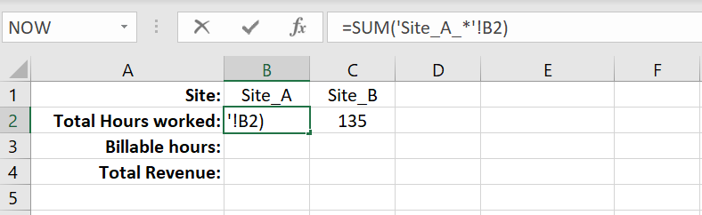
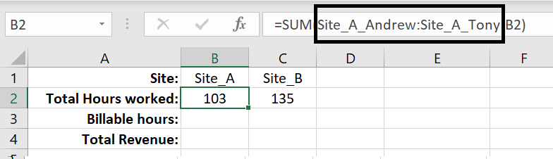
After we press Enter, Excel will automatically update the formula to include all sheets that starts with “Site_A_”:
The benefit of this is that the order of the worksheets does not matter here. In the section above, we need to start with the first worksheet on the left and end with the last worksheet on the right. With the use of wildcards, Excel automatically captures all worksheets that have that particular word/term in their names.
Wildcards are not restricted to being used at the end. We can use them in the beginning. Using the very first example we have, the worksheets with “Monday” to “Friday”, because each worksheet has “day” in it, we can use 3D Range with wildcard in that situation too:
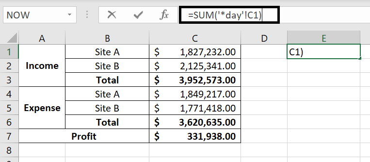
=SUM(‘*day’!C1)
After we press Enter, Excel will automatically update the formula to include any worksheets that has “day” at the end in their names:
What To Be Mindful Of…
There is a few things we should keep in mind when using 3D ranges:
Moving Worksheets Around Afterwards
When we refer to a range of cells, say A1:A20, and then we add a row in between, Excel will automatically update the range to A1:A21. Well it’s the same for 3D Ranges. After we’ve entered the formula, regardless whether we used wildcards or not, if we then add a worksheet in between the worksheets, they will be included. Let’s use the example above with “Site_A_”:
We used a wildcard with “Site_A_” and this is what Excel returns:
If we then add a worksheet between ‘Site_A_Andrew’ and ‘Site_A_Tony’, even if the worksheet’s name does not have ‘Site_A_’, it will still be included. And in this case, we’ve put a ridiculously large number in the ‘Random’ worksheet to illustrate the change:

Adding A New Worksheet Afterwards
Following on from above, it does also mean that when we use a wildcard in a 3D Range, e.g. with ‘Site_A_’ above, if we then add a new worksheet with ‘Site_A_’, the formula will not pick up the new worksheet unless we move that sheet in between the 3D Range already created. For example, we created a ‘Site_A_Random’ and we can see that the total in ‘Summary’ did not get updated at all:
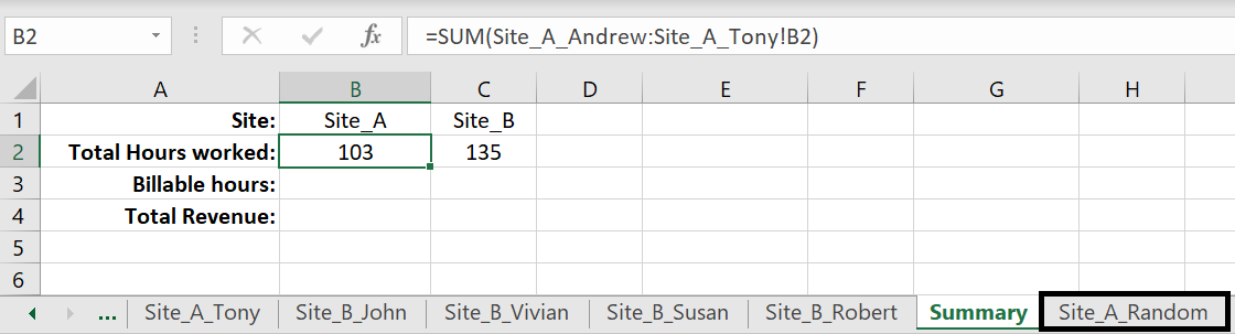
This is because ‘Site_A_Random’ is outside ‘Site_A_Andrew’ and ‘Site_A_Tony’. To include ‘Site_A_Random’, we will need to move that sheet in between ‘Site_A_Andrew’ and ‘Site_A_Tony’.
All Worksheets Must Use the Same Template
One last reminder: because we are referring to the same cell across multiple worksheets, it is important to make sure all sheets follow the same layout, format and template. Otherwise we could be adding the wrong values together.
0 Comments Leave a comment