Getting different errors in Excel? Error messages can be frustrating but they are also extremely useful. And thank goodness they are here. Imagine if we made a mistake and Excel does not tell us about it.
| IFERROR (use with caution) Before we go into the common errors we see in Excel, let’s go through how we can manage and handle these errors. IFERROR function lets you decide what you want to see returned if there’s an error with the function. The formula is very simple to use: =IFERROR(formula, value to return if error). It is important to remember that this formula does not fix or solve the error for us. In fact it just helps us hide it. Of course there are situations this formula can be very useful. For example as we can see below, VLOOKUP will return #NA if the lookup value cannot be found. An easy way to tidy up would be: =IFERROR(vlookup, “cannot be found”) as the note “cannot be found” will most likely be more informative than #NA. |
#NA
#NA means “no value is available”. This error appears when something cannot be found. It happens most often in VLOOKUP and MATCH functions when a referenced value cannot be found.
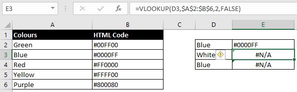
- “White” is not in the list of colours in the table and hence there is the #NA error
- With the second example, blue is in the table but VLOOKUP function is showing the #NA error. This is a common error and it is because there is a space after blue: “blue “.
- Using the TRIM function can remove space in the beginning and end of a text
- Setting up dropdown boxes will limit what users can put in the referenced cell.
#VALUE
#VALUE means there is something wrong with your function. This error message is fairly broad and can be a result of a number of different scenarios. The easiest and quickest way would be to see below which formula you are using:
VLOOKUP
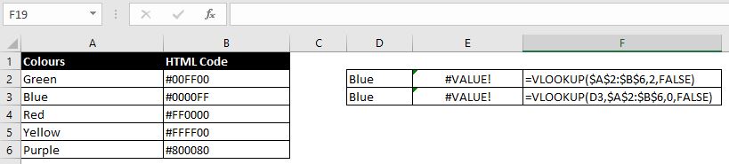
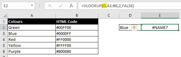
- With the first example, the lookup value is missing in the beginning. Purpose of VLOOKUP function is to look at ONE referenced cell and matches it with the list of cells in the left column in the table. In example above, the table has become the lookup value. VLOOKUP cannot look for a whole array of cells in a table. One at a time.
- Solution: add the correct lookup_value into the formula:
=VLOOKUP(D2,$A$2:$B$6,2,FALSE)
- Solution: add the correct lookup_value into the formula:
- #VALUE can appear in VLOOKUP function when your column index number is 0 or if your column index number is higher than number of columns in the table you referenced. E.g. in above table, we have referenced A2:B6 which has two columns. #VALUE will appear if we put column index number as 3 (or above).
Addition/Subtraction/Multiplication/Division
This happens when the formula references a cell that is not a number.
Sometimes even when a value in a cell looks like a number, Excel may not necessarily recognise it as a number. E.g. if there are other characters in the cell (“11,33” or “111,”) or if there are spaces within the number (“12 345” or “12345.5 6”). Easiest way to check is to use the ISNUMBER function on the cell. If function returns TRUE, Excel recognises it as a number. If it returns FALSE, Excel does not recognise it as a number.
#REF
#REF appears a cell or an array of cells referenced is not valid. This happens most when a cell or an array of cells is deleted. And this happens when we delete current data in the file and replace it with new set of data. In Excel there is a difference between deleting cells and clearing cells. Clearing cells only remove content in current cells while deleting cells would delete them (and shift adjacent cells accordingly)
- Best way to avoid this is to get into the habit of clearing content, not deleting cells.
- Best way to fix this would be to quickly undo. Otherwise we would have to go into the formula and fix the #REF by referencing the right cell(s) again.
#NUM!
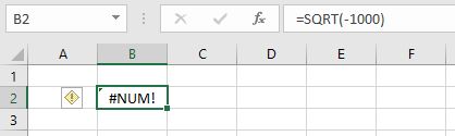
As the name of the error message suggests, #NUM! appears when there is a problem with the number in the formula. It often happens when the function cannot find an answer. Here are some of the common scenarios:
- Square root of a negative number:
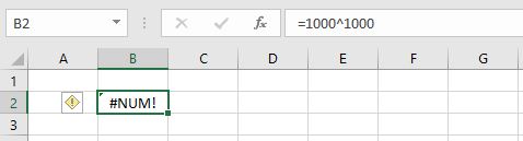
- Result is too big or too small: the largest number you can have in Excel is 1 with 308 zeroes after it. Try this in Excel. You can enter =10^308 into Excel but if you enter =10^308, you will get #NUM. This is the same if you use -10 instead of 10. Hence #NUM can also appear when number is too small:
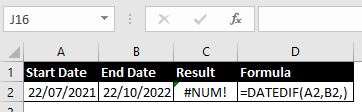
- Missing Information in Formula which has made the formula impossible to be calculated. For example the function DATEDIF calculates the difference between two dates but we must specify whether we want to calculate the difference in years, months or days. And we specify this in the formula: =DATEDIF(start date, end date, days/months/years). If we leave the third value blank, we get a #NUM:
#NAME
There can be a few reasons why #NAME appears:
- Typo in formula or function name:
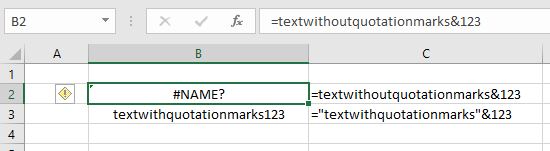
- Quotation missing for text in a formula:

- Named reference does not exist:
- One way to make sure we don’t mistype the named reference in a formula is to press F3 instead of typing the named reference ourselves. By pressing F3, we can see the list of named references and select from there
- Check in Formula > Name Manager to make sure the named reference was actually created
- Check your spelling
#NULL!
Check to make sure there is no unnecessary space in formula and there’s no typo with comma “,” or colon “:”. Here are some examples where formulas return #NULL!:
- =SUM(D7 D16) – colon missing between D7 and D16
- =SUM(C7:C16 D7:D16) – comma missing between C16 and D17
- =D7+D8 D9 – space in between D8 and D9. The space needs to be replaced by a mathematical operator such as a plus or minus sign
Circular Referencing
Circular referencing occurs when calculation in the formula includes the current cell. This creates an infinite loop. For example: A3 = A1 + A2 + A3. With circular referencing, Excel will always prompt you with the following message:
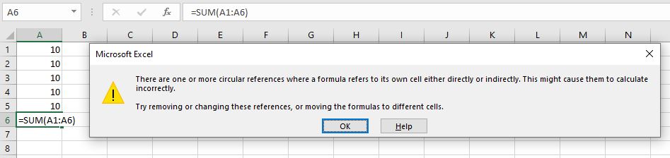
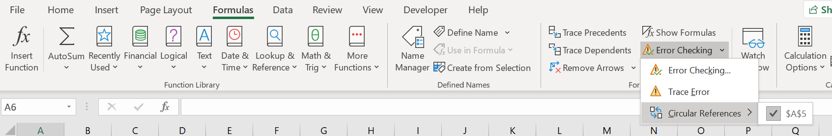
But in case you clicked “Ok” without reading the message, circular referencing will be more difficult to detect. Instead of displaying a more obvious error message, it will return 0 as a result. You can also check for circular referencing by clicking on:
- Formula tab > Error Checking (in Formula Auditing section) > Circular Referencing
#DIV/0
The error message itself is self-explanatory. This happens when we want to divide a number by 0. When we divide A by B, we are splitting A into B number of parts. The reason why we cannot divide by 0 is simply because no matter how we divide or split something, we can never turn something into nothing (0).
#SPILL
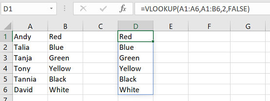
#SPILL appears when the result in formula has to go across multiple cells but some of those cells already contain data. This can happen with formulas that have lookup_value in the function such as VLOOKUP and MATCH. As an example, with VLOOKUP, Excel allows us to put a range of cells as the lookup_value and it will calculate the results for us in multiple cells. See below:
However if we have data already in Cells D2 to D6, they will block Excel from giving us the result for the VLOOKUP:
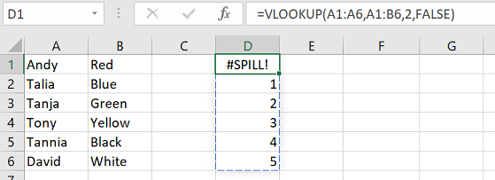
Easiest way to fix this error is to clear the data in those cells so nothing is in the way of the results.
######
This appears when column width is not wide enough to display the value in the cell. The easiest way to check is to widen the column width and see if the error message disappears.
Has This Page Answered Your Question?
There are many different errors in Excel. We hope this page has helped you resolve your problem. If not, can you let us know what it is and we will add it onto the page!