Can you use Excel without power query? Yes. But can you use Power Query in Excel to simplify and automate any formatting and reporting processes that you do every week or every month? Answer is also yes. It is definitely worth spending time setting up Power Query.

We will first go through a simple illustration of how Power Query works from start to end. And then we will go through various editing/transformations we can do before loading the data.

• Power Query
• Transforming/Editing Data
  • Splitting Columns
  • Calculate Day of the Week From Date
  • Filtering Columns
  • Conditional Formatting (IF function)
  • Editing the Applied Steps
• Combining/Merging data
• Extracting File Names and Path Directories

Setting Up Power Query in Excel

Power Query allows us to query data from various sources, edit the data (e.g. combining data across multiple sources, splitting/adding columns, filtering), load the data onto Excel and create Pivot Table/Charts from it. Similar to Macro, the series of steps is recorded in the query and we can run the query again with new data (for example when next month’s report). We can also add/remove/rearrange/edit the steps easily if required.

Querying and Loading the Data

We can begin Power Query by choosing the relevant data source. Go to Data > New Query. We can create a new query from various sources such as workbook, CSV, text file, XML or Folder:

Which file should I choose? It is important to pick the right file here. If we are going to add new data files on a regular basis, it will be best to create a folder and save all the files there. See image on the left: In this case, we should create a new query from Folder. When we add new files into the folder, it can be updated easily by refreshing the data. If we are working with one data file and that one data file gets updated regularly, then we should create a new query from workbook or CSV depending on the file type. Note: make sure you first check if your file is an Excel workbook or a CSV.

In this case, we will use the example above and create a new query from Folder. Go to Data > New Query > From Folder. Here we can copy and paste the directory path or you can browse for the folder:

After we click Ok, we can then see the list of files in that folder. In this section, we will not edit/transform the data. For information how to edit/transform data, please go to next section – Transforming Data. Here we will simply combine & load the data.

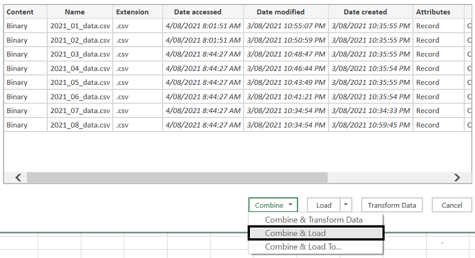
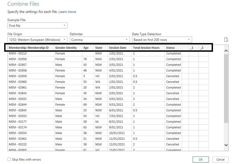
A preview of the data in your files will appear.

Click Ok. And Excel will load the data into a table format. Quickest way to make sure the data has loaded correctly is to use the filter in Source.Name column and check that all data file names are there:

Once we are happy with the data in the table, we can create Pivot Tables with the relevant information. In this section, Pivot Tables and Power Query make a great combination. Because same as Power Query, once Pivot Tables are set up, they can be updated and refreshed easily with click of a button.

Loading New Data

Now that we have created a query from the folder path, it is very easy to update new data. All we have to do is:

1. Download a new report
2. Save in the same folder
3. Click Refresh in the Excel file

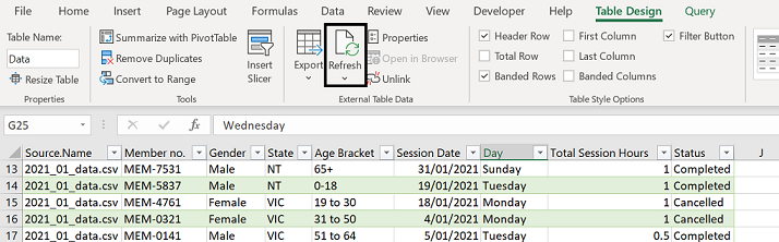
And ta da! We can see the new data is now in here:

Transforming/Editing Data

Prior to loading the data, we have the option to format the data first. Similar to Macro, the series of steps is recorded and will run again when query is refreshed. The series of steps can also be edited. To edit the data before loading:

Splitting Columns

1. Select the column we would like to split
2. Go to Transform tab at the top
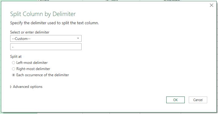
3. Select Split Column > By Delimiter
4. Select delimiter option: in the example below, we will select Custom and enter “-“

And this will be the end result:

Day of the Week

1. Select the column with dates
2. Go to Transform tab at the top
3. Select Date > Day > Name of Day

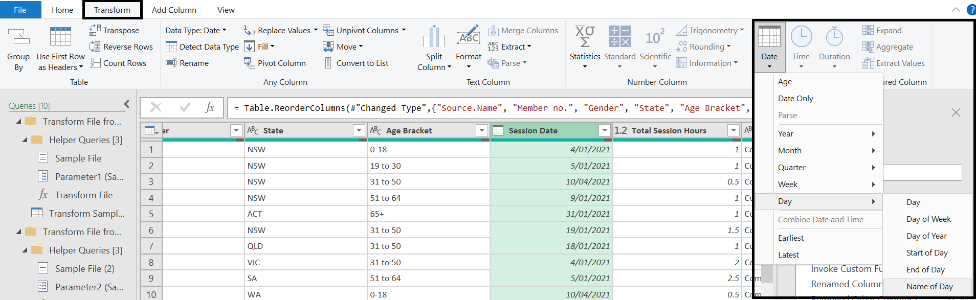
And this will be the result:

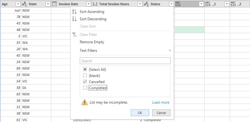
Filtering Columns

Simple filtering can be very helpful in removing irrelevant information before loading the data. Don’t forget: the more we can automate here the more time we will save in the future.

1. Select relevant column
2. Deselect the data we want to remove

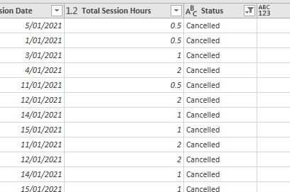
In this example, let’s say we want a report on session cancellation:

And this will be the result:

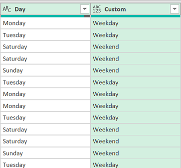
Conditional Formatting

Note: this can be used like an IF function

1. Go to Add Column tab
2. Select Conditional Column
3. Apply the relevant conditional formatting

In the example below, we will group all our members into age brackets:

And this is the end result:

Editing the Applied Steps

Combining/Merging Data

We can merge merge files together as long as the files have common data that can connect them together. For example we could have monthly sales reports and also a master file on employee/client details.

1. Load the first set of data
2. Load the second file
3. Right-click on one of the queries in Workbook Queries on the right (see below)
4. Select Merge
5. Select the second set of data you would like to merge in the second dropdown box (see below)
6. In both set of data, select the columns which match and connect the two data sets together
7. Click Ok
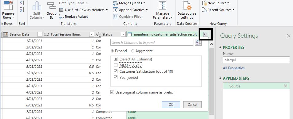
8. Select the columns you would like to merge into the first set of data
9. Close & Load

Steps 3 & 4:

Steps 5 to 7

Step 8

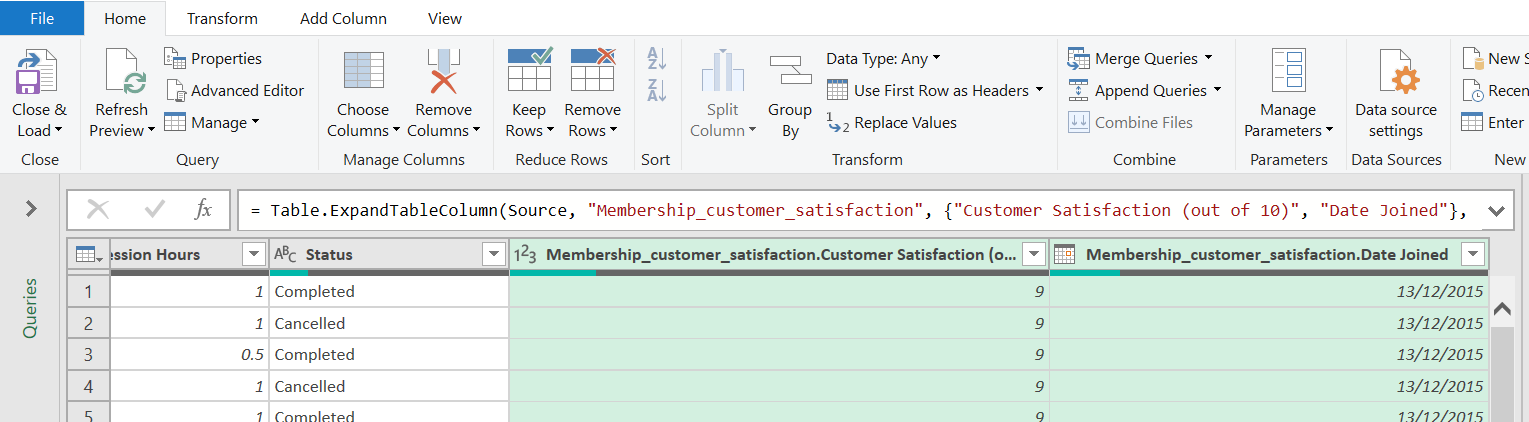
And this will be the new table:

Extracting File Names and Path Directories

An easy way to extract file names and folder path directories within a folder is to create a Power Query from the folder.

1. Go to the Data tab > New Query > From File > From Folder
2. Either paste in the folder path or browse
3. Select Load (Note: make sure we don’t select Combine here)

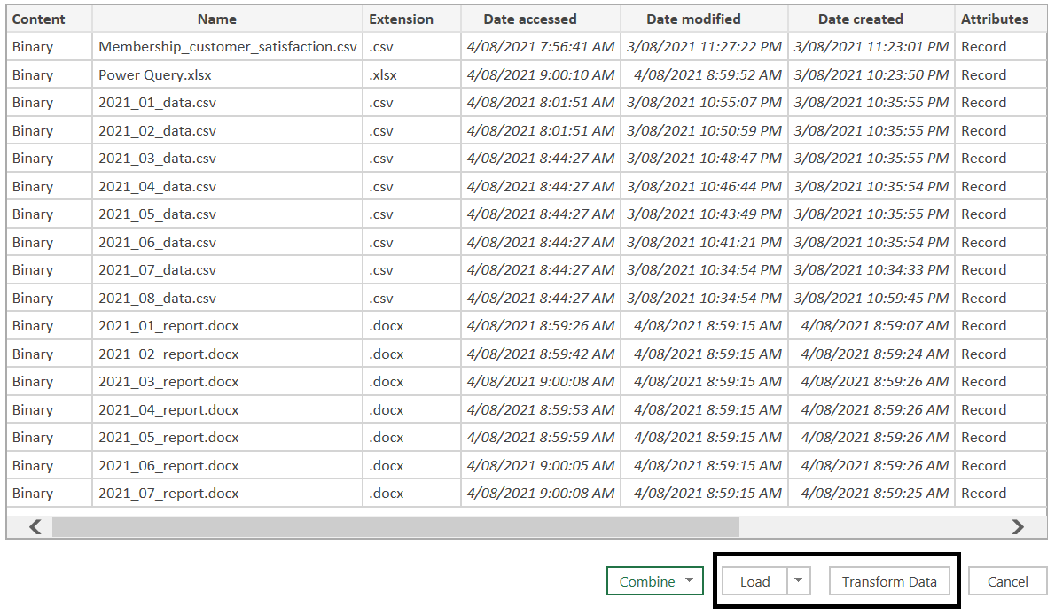
Once we finish editing, click on Close & Load and we will have a list of every file names within that folder (and its subfolders) and also the folder path directory each file is in.