What is a simple way to identify duplicates in Excel? In this article, we will go through two ways of doing that: using Conditional Formatting and COUNTIF function. And at the end we will look at how we can find the total number of unique values in a list.

Finding Duplicates with Conditional Formatting

The easiest way to finding duplicates in a column is to use conditional formatting:

1. Highlight the column
2. Go to Conditional Formatting > Highlight Cells Rules > Duplicate Values
   
   
   
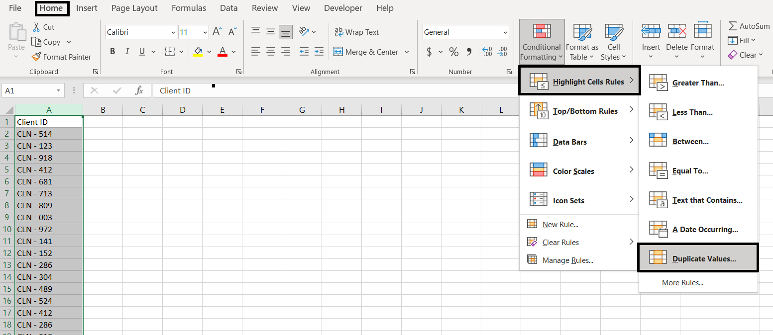
3. Select the formatting we want for cells that contain duplicates
4. Click OK

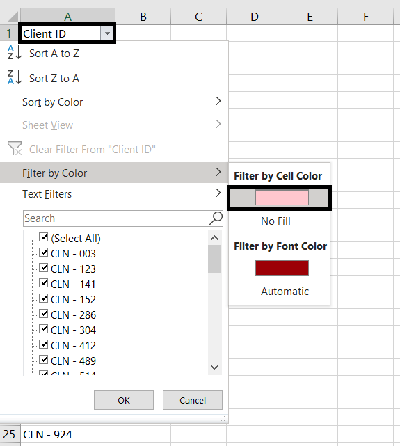
After conditional formatting is applied, we can add Filter to the column and filter by cell color:

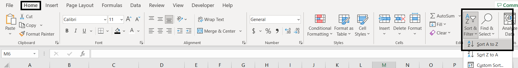
And then we can do the cleaning up we need. We can start from the top and delete each duplicate row. But before doing so, we suggest sorting the data in order first. You can do that by going to the Home tab > Editing section > Sort & Filter > Sort A to Z:

Why do we need to do this? We want to sort the list in order first so then we can group each set of duplicates together. This is not a mandatory step but it does make it very clear how many duplicates there are for each item and hence gives us an indication on how many duplicated row we will need to remove for each.

Note: when deleting duplicates, do not delete more than one row at a time because we only want to delete the duplicated cell. The idea is when we delete/clear one cell, because there will be no more duplicate (assuming there is only one duplicate), the conditional formatting for the second cell will disappear.

Finding Duplicates using COUNTIF function

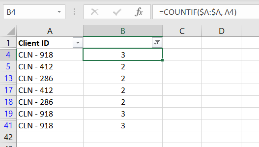
Conditional formatting certainly helps with identifying the duplicates but it does not tell us how many duplicates there are for each cell. This is something the COUNTIF function can do:

=COUNTIF($A:$A, A2)

Because we are counting that item which is inside the list itself, the COUNTIF function will not return a number lower than 1. So if we want to precisely calculate how many duplicates there are for a particular value, we can add a “- 1” at the end of the formula. For example above: “=COUNTIF($A:$A, A2) – 1”. Afterwards we could apply Filter and filter out values that have no duplicates:

Counting Unique Values

Above is the most common method we use to identify duplicates. To then count the number of unique values, we usually do one of the following:

Copy the column and paste it on another sheet. Having the column highlighted, go to Data tab > select Remove Duplicates: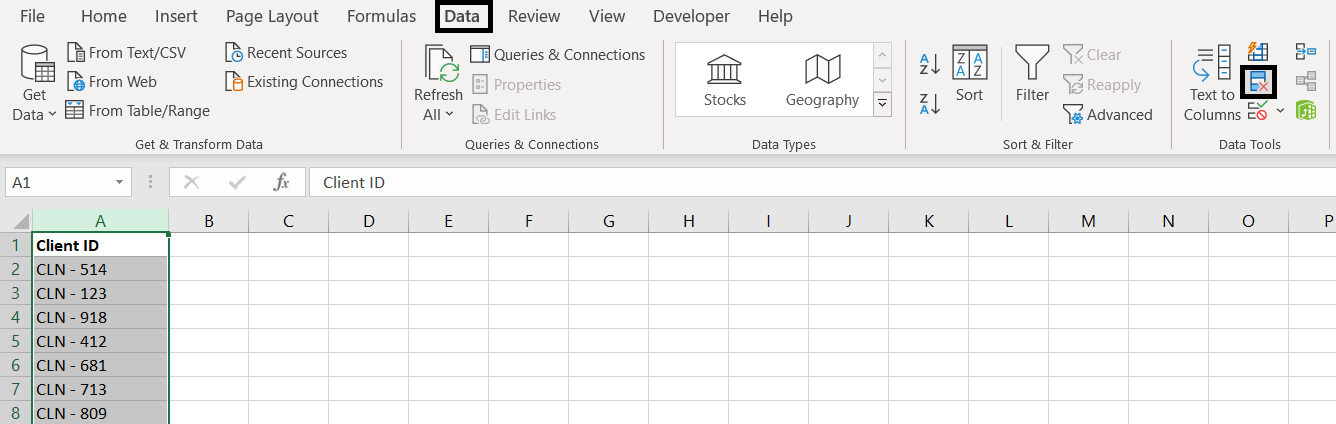

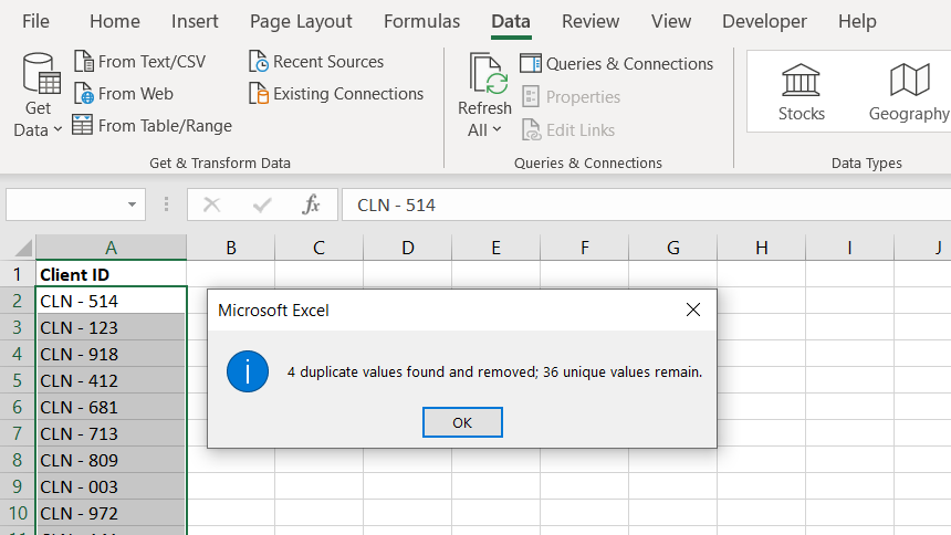
And Excel will tell us how many unique values there are in the list. We can see below Excel has very cleverly excluded the heading of the column so we know the 36 does not include the heading.

Have we missed anything on this topic? If you find that we have missed anything, or if you have any questions, want us to include anything else into this article or need clarification on anything here, please let a comment below! We want to keep improving our content so it is useful for everyone.