Count the Number of Unique Values

Do you have a list of data that has some duplicates in there and you would like to count the number of unique values in the list? This is what we will go through in this article. We will go through two different ways to do this – 1) Remove duplicates and 2) with a formula. As always with Excel, there’s more than one way to do anything. Another method you may have seen on the internet is:

• To count how many of each value there is in the list and convert them into a fraction (1/x). And then we add all the fractions together. It really is a very smart and brilliant way of solving the issue. The idea is that if there is only one of that entry in the list then the fraction will just be 1/1 which is 1. If there are two, then the fraction will be 1/2 and 1/2 and the two duplicates will add up to 1. And if there are three duplicates, each fraction will be 1/3 and again the three duplicates will still add up to 1. So the logic is as long as we convert each “count” into a fraction, each set of duplicates will add up to 1 so we can get a list of unique values. This is not a method we will go through extensively in this article but here’s an example below:
  
  
• 
  And there are 7 unique values in Column A: 3, 4, 5, 6, 7, 8, 9.

Remove Duplicates

This is most likely the most simple way to count how many unique values there are in a list. In the Data tab at the top, there is a Remove Duplicates function and we will make use of that.

1. Copy the relevant array or range of data
2. Paste it into a separate column that does not already have data in there – this is so that we will not change the original data
3. Go to Data tab at the top
4. Click on Remove Duplicate
   
   
5. Click OK
6. And we will see how many unique values there are in the message box:
   
   

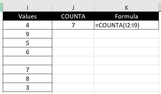
Be careful if there are blanks in the list. For example below:

There are only 7 numbers but the blank is counted as a value so Excel is saying there are 8 unique values. If we do not want blanks to be counted, to be absolutely sure and accurate with the number of unique values, we can then use COUNTA function to identify the number of values in the new list:

Counting Unique Values with a Formula

Using “Remove Duplicates” then COUNTA function is one way to count the number of unique values. But it may not be the most ideal approach for you. After all it is quite manual. You’ll need to copy the data and paste it into a column which doesn’t already have any data. And the adjacent (to its left and right) columns cannot have any data. You cannot update the data and get an updated result instantly. Every time you update the data, you need to follow the same steps again. So how can we count the number of unique values with just one formula?

In the very beginning of this article, we mentioned one way of doing this in a formula. That is to use the COUNTIF function, convert each result into a fraction and then use SUM to add all the fractions up. You’ll most likely find this approach very common across the internet.

But as we mentioned, there’s always more than one way to solve an issue in Excel. And here we will explore another method. The best way to approach this sort of problems (ones which there is no built-in Excel formula for) is to approach the issue logically. Ignore Excel and just think about the situation logically. We have an array of random values here and some are duplicates. How can we work out how many unique values there are? You might be able to think of a completely new approach and come up with your own formula and method. Anyway here’s how we will do it:

One way to count the number of unique values in a list is:

• We will first sort the array in order. In this sorted array, we will go down the list from top to bottom. If the current value is not equal to the one below it, it counts as a unique value and will count as 1. If the current value is the same as the one below it, it is a duplicate and will count as 0.

The formula is:

• =SUM(IF(INDEX(SORT(array),ROW(array),1)=INDEX(SORT(array + one row),ROW(array)+1,1),0,1))
  
  E.g.: =SUM(IF(INDEX(SORT(A1:A25),ROW(A1:A25),1)=INDEX(SORT(A1:A26),ROW(A1:A25)+1,1),0,1))

We will not go through the INDEX function in detail in this article. To find more information on INDEX function, you can have a look at our article here: Index and Match – A More Advanced Lookup. As a quick summary, the function of an INDEX formula is to locate a particular value in an array based on the relevant row and column numbers we provide. So here we go, let’s break down the formula above:

• INDEX(SORT(array),ROW(array),1): this part of the formula first sorts the array in order and then picks out each cell one by one starting from first row. And it will always look at column 1 since we have a list of data all in the same column here.
  
• INDEX(SORT(array + one row),ROW(array)+1,1): this part of the formula is very similar, except for two changes and you might have already picked them out:
  
  1. the “+1” at the end – this is to make sure whatever cell we are looking at in the first INDEX function, in this INDEX function we are looking at the cell directly under it. Hence the “ROW + 1”.
     
  2. the “array + one row” – the reason for the extra row in the array of data is because for every cell in the first INDEX function we are comparing it with the cell right under it. Hence we will need that extra row in this INDEX function so that with the last cell in the first INDEX function, we have an extra cell in this INDEX function for it to compare with.

• The rest of the formula is more self-explanatory. The next part is to wrap them in an IF function so that if the cell is the same as the cell directly under it, then the IF function will return 0 because it’ll be a duplicate. And return 1 if they are not the same because it’ll be a unique value. At the end we wrap the whole formula together with a SUM function to add all the 1s (and 0s) together.

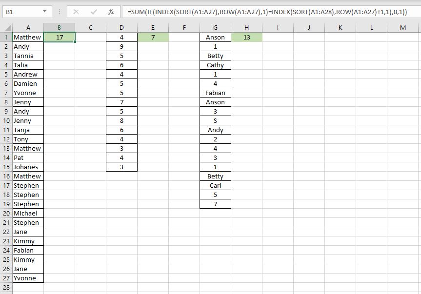
Let’s go through this with an example. Here we have three sets of data. First one is all numbers. Second one is all texts. Third is a mixture:

Essentially the formulas across the three are all the same regardless if it is all text, all numbers or a combination. The only difference is the array:

• =SUM(IF(INDEX(SORT(A1:A27),ROW(A1:A27),1)=INDEX(SORT(A1:A28),ROW(A1:A27)+1,1),0,1))
  
• =SUM(IF(INDEX(SORT(D1:D15),ROW(D1:D15),1)=INDEX(SORT(D1:D16),ROW(D1:D15)+1,1),0,1))
  
• =SUM(IF(INDEX(SORT(G1:G19),ROW(G1:G19),1)=INDEX(SORT(G1:G20),ROW(G1:G19)+1,1),0,1))

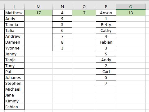
Let’s check our work with the first method we went through – Remove Duplicates and COUNTA:

And we get the same results. Simple enough? There is a catch to it. So far we’ve only examined situations where the data starts from the first row. What happens when we shift the data above to start from row 2 for example? We get a #REF.

In the example we will go through what we need to update in the formula (and what we don’t need to update):

Formula:

• =SUM(IF(INDEX(SORT(A2:A28),ROW(A1:A27),1)=INDEX(SORT(A2:A29),ROW(A1:A27)+1,1),0,1))
  
• SORT(A2:A28) & SORT(A2:A29) – Both array reference in the two INDEX functions need to be updated. The array is now situated at A2:A28. And following the same logic as above, the second array needs to be A2:A29 to accommodate the last cell in the first array – i.e. when it gets to A28 in the first INDEX function, that cell will be compared with A29 in the second INDEX function, hence the array in the second formula needs to be A2:A29.
  
• ROW(A1:A27) & ROW(A1:A27)+1 – Maybe the more surprising thing is that the two arrays for the row numbers don’t need updating. Let’s take a step back and remember the INDEX function – INDEX(array, row number, column number). Row numbers and column numbers are references relative to the array. For example: INDEX(A1:C10, 3, 2) is referring to the third row and second column in the array A1:C10. If we update the ROW formula to ROW(A2:A28), this means the row numbers will start from 2 and end at 28. But remember our array, although has now moved down by one (A2:A28), the number of rows hasn’t actually changed. Meaning it still has 27 rows so we go through row 1, 2, 3, 4…27 gradually in A2:A28. And not start from 2 to 28. Put it this way, starting with 2 would mean INDEX(SORT(A2:A28), 2, 1) which means we will be starting with A3. And INDEX(SORT(A2:A28), 28, 1), this will give us an error because there are only 27 rows in the array A2:A28. And if you are curious, the reason why the second INDEX function also looks from row 1 to 27 although the array (A2:A29) has 28 rows is because we have the +1 at the end of the ROW function.