SUMPRODUCT Function

SUMPRODUCT Function – What Can It Do?

October 31, 2022
Excel formulas

If you don’t use Excel very often, you may not be familiar with the SUMPRODUCT function. Or you may not even heard of it. And even for those who have heard of it and know the basics, this function has other applications which may not be obvious at first sight. In this article, we will examine what the SUMPRODUCT function can do and what makes it unique.

Before going through examples, we will first explain how the SUMPRODUCT function works. With this function, we need to enter array(s) into the formula:

=SUMPRODUCT(array1, [array2], [array3],…)

What the SUMPRODUCT function would do is to:

Multiply the first value(s) of each array together and then multiply the second value(s) of each array together. And the third and fourth and so on…depending on how many numbers there are in the array(s). At the end, SUMPRODUCT will add all the values together:

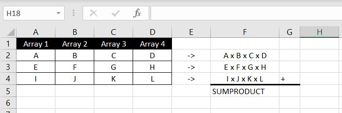
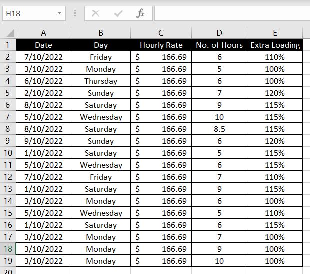
Here’s a simple example. In Column B, we have the team member’s hourly rate and in Column C, we have the number of hours worked. In Column C, we have the extra loading the team member receives:

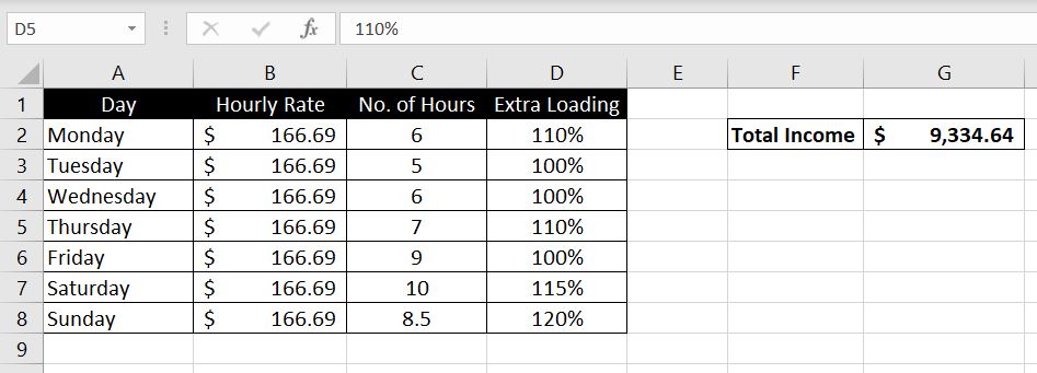
=SUMPRODUCT(B2:B8,C2:C8,D2:D8)

Here we entered three arrays: 1) B2:B8, 2) C2:C8, and 3) D2:D8. The SUMPRODUCT function would then calculate B2 x C2 x D2…B3 x C3 x D3…B4 x C4 x D4…and so on. And at the end, the function would add all the values together and this will be the result the SUMPRODUCT function returns at the end.

We can see when this function could be useful. But at first sight, it seems like this function is only a shortcut for multiplications and addition. It’s actually much more than that. We will now look at what other ways this function can be used.

SUMPRODUCT…COUNTIF?

To start with the basics, SUMPRODUCT can be used as a COUNTIF function. It’s simple, we will just need to be mindful of the syntax. We need to specify the array and what we are looking for. What may surprise most people is that in addition, we will also need to input some arithmetical operations into the SUMPRODUCT function. When the function goes through the array to search for the lookup value, the function returns a TRUE or FALSE result. By adding mathematical operations within the function, Excel knows to treat TRUE as 1 and FALSE as 0. There is a couple of ways this could be done. We could add:

*1 : which is to multiply the result by 1. A TRUE result (1) will remain as 1 (1 x 1). A FALSE result (0) will remain 0 (0 x 1), or
— : very similar to above, the two negative signs (–) mean we have -1 x -1 which will be equivalent to multiplying by 1

Here’s an example below:

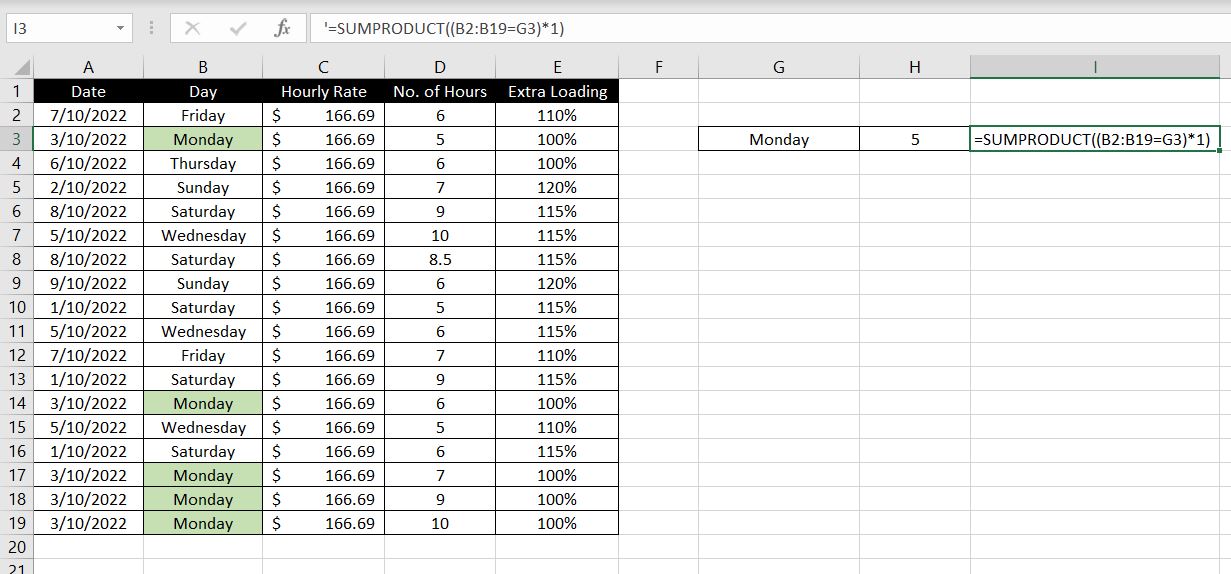
=SUMPRODUCT((B2:B19=G3)*1)

First we specify the array (B2:B19) and we want to check how many “Monday”s (G3) are in the array. And finally we multiply that by 1. Note: it is very important to put a bracket around the condition before multiplying by 1. Alternatively this would yield the same result:

=SUMPRODUCT(–(B2:B19=G3))

SUMPRODUCT….IF?

Building on from above, we can then set conditions into our SUMPRODUCT formulas. For example, with above, we could calculate total income but only for sessions that fall on Mondays. Remember, for each condition met in the array, the SUMPRODUCT function will return 1. Hence with the example above, all we have to put in the function is:

Condition x Hourly Rate x No. of Hours x Extra Loading

This is because if condition is met, SUMPRODUCT will return 1, hence:

1 x Hourly Rate x No. of Hours x Extra Loading

If condition is not met, SUMPRODUCT will return 0, hence:

0 x Hourly Rate x No. of Hours x Extra Loading = 0

Let’s have a look at the example below:

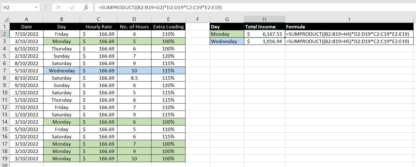
=SUMPRODUCT((B2:B19=H4)*D2:D19*C2:C19*E2:E19)

=SUMPRODUCT((B2:B19=H5)*D2:D19*C2:C19*E2:E19)

The formula looks a bit long but it’s not too complicated. The “*D2:D19*C2:C19*E2:E19” part is similar to how we use any SUMPRODUCT function. In this case, it is:

Hourly Rate x No. of Hours x Extra Loading

And we multiply that with the condition we want to set – “(B2:B19=H4)“. As explained above, if condition is met, SUMPRODUCT will return 1. If condition is not met, SUMPRODUCT will return 0.

The key difference here is that in the first example, we separate each array in the function with a comma (,):

=SUMPRODUCT(B2:B8,C2:C8,D2:D8)

But once we add condition(s) into the formula, we need to specify that we want to multiply (*) the values together:

=SUMPRODUCT((B2:B19=H4)*D2:D19*C2:C19*E2:E19)

SUMPRODUCT…OR?

So what makes SUMPRODUCT function unique? One of the biggest differences is that with COUNTIFS or SUMIFS, Excel will only count or add if ALL conditions are met. With SUMPRODUCT, we could use the function to calculate COUNTIFS and SUMIFS, except we don’t need ALL conditions to be met. We can get SUMPRODUCT to calculate as long as one of the conditions is met.

As an example below:

Unless we add multiple COUNTIF formulas together, we cannot use COUNTIF to count the number of Mondays and Wednesdays in Column B. But we can do that easily with SUMPRODUCT:

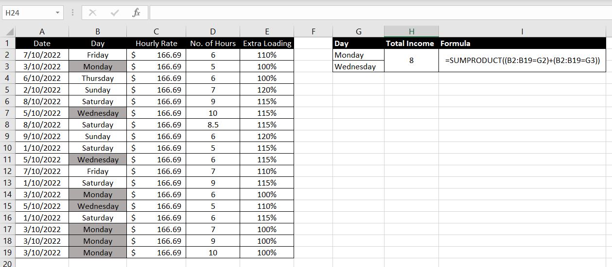
=SUMPRODUCT((B2:B19=G2)+(B2:B19=G3))

This follows very similar logic to what we had above. All we need to do is put a bracket around each of the condition and add them together. For any field in Column B that is a “Monday”, the formula will return 1 + 0. And for any field that is a “Wednesday”, the formula will return 0 + 1. For any other field, the formula will return 0 + 0.

We can also require SUMPRODUCT to calculate only when ALL conditions are met. In this example below, we want to calculate the number of sessions that fall on a Monday and is for a duration of 5 hours:

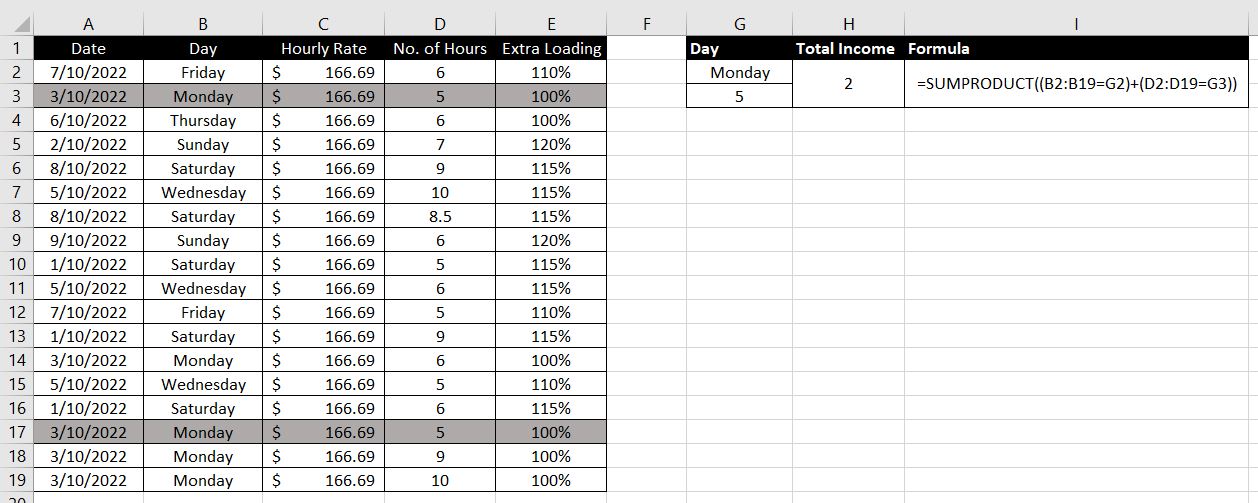
=SUMPRODUCT((B2:B19=G2)*(D2:D19=G3))

In this case, we want to multiply the conditions together instead of adding them:

If a session falls on a Monday and is 5 hours, SUMPRODUCT will return 1 x 1 = 1
If a session falls on a Monday but is not 5 hours, SUMPRODUCT will return 1 x 0 = 0
If a session does not fall on a Monday but is 5 hours, SUMPRODUCT will return 0 x 1 = 0
Any other session will simply be 0 x 0 = 0

This means only sessions that fall on a Monday and are of 5 hours will return a 1 and will be counted. Any other session will return a 0 and won’t be counted.

As you can imagine, we can be very creative when using SUMPRODUCT. The function is definitely not as simple as it seems. And it can be applied in many more situations than people would generally expect.

We will go through one more example. In this case, we will calculate total income for sessions that fall on a Monday OR Wednesday:

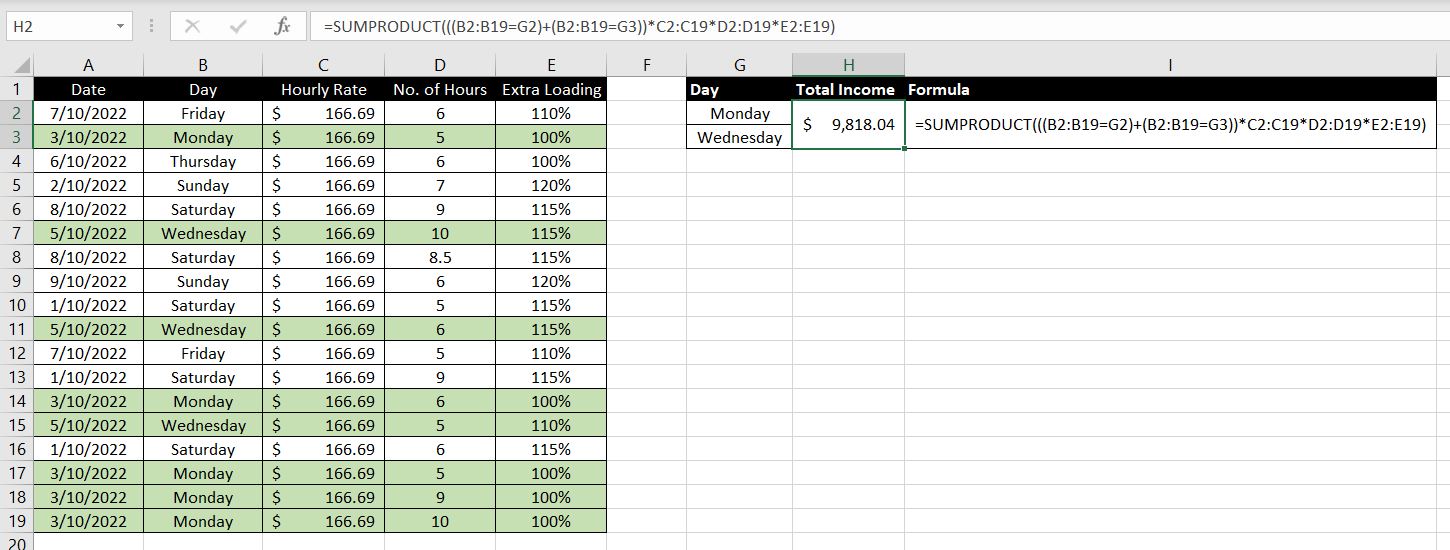
=SUMPRODUCT(((B2:B19=G2)+(B2:B19=G3))*C2:C19*D2:D19*E2:E19)

Once again the formula may be long but it is not complicated. We will break it down into its components:

((B2:B19=G2)+(B2:B19=G3)) – this is the condition that the value in B2:B19 will either need to be a “Monday” or “Wednesday”. Either one would return a 1. Any other day would return a 0 and hence be excluded
C2:C19 – Hourly Rate
D2:D19 – No. of Hours
E2:E19 – Extra Loading

And we multiply them all together so we join them together with the multiplication sign (*)

What To Be Careful With

There is a couple of things we need to be careful with when using SUMPRODUCT function:

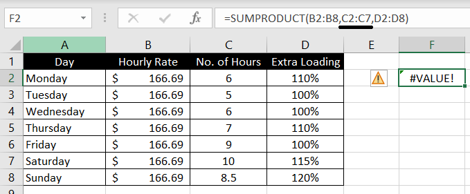
#VALUE – the number of values in each array needs to match. When they don’t, Excel will return a #VALUE error:
When cells in an array are blank, Excel treats those blank cells as 0:

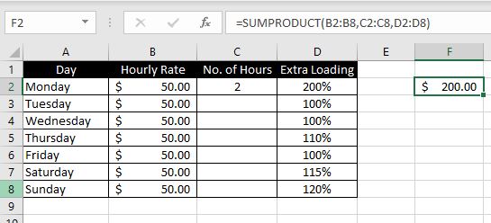
The first values of each array multiply to return 200 (50 x 2 x 200%). The rest of the values in Column C are 0. Hence it becomes 200 + 0 + 0 +0 +0 +0 +0 = 200.

We hope you find this article useful. If you have any additional questions on SUMPRODUCT function, feel free to leave a comment below!