When we download reports from CRMs and various systems, we can’t always control how the data will be presented. Luckily we have Excel. In this article, we will go through functions such as RIGHT, LEFT, FIND, MID and how to use these functions together to extract part of a text within a cell.
RIGHT, MID & LEFT Functions
Before combining various functions such as RIGHT, LEN, FIND together, we will first go through the RIGHT, MID and LEFT functions in Excel. And we will do so using a few examples.
RIGHT & LEFT
The RIGHT function in Excel allows us to extract the part of a text within a cell, starting from the cell up to the nth character. The function is:
=RIGHT(text, [num_chars])
- Text: the text or cell reference you would like to extract text from. Note that you don’t actually have to refer to a cell, you could write =RIGHT(“Kelvin”) in which case this formula will return “n”.
- [num_chars]: starting from the right, the number of characters you would like to extract. Note that this is in square bracket, this means input for this field is optional. If nothing is entered (e.g. =RIGHT(“Kelvin”)), the formula will by default return one character from the right which is really the last character in the string
The LEFT function is very similar. Instead of starting from the right, it starts on the left.
We will go through a few examples below which will highlight the differences between the two:

The functions are fairly simple to use. Below, we will explore what happens when we insert a negative number for [num_chars] or a number that is larger than number of characters in the text:

As we can see, if we ask Excel to return more characters than what’s in the original text, Excel will just return the full text. And if we enter a negative number, Excel will return with an error #VALUE.
MID
The MID function is quite similar to the LEFT function except we can specify where the starting position should be. Once we specify the starting position, Excel extracts x numbers of characters to the right from that position. And no we cannot use negative numbers to extract strings that are to the left of the starting position. Putting a negative number for [num_chars] will again return the #VALUE error.
The MID function is:
=MID(text, start_num, num_chars)
Straight away we see the difference between MID and RIGHT/LEFT. There is no square brackets around any of the fields. This means all fields are mandatory. If we do not enter a number for num_chars, we will get a message from Excel saying “You’ve entered too few arguments for this function”
- Text: the text or cell reference you would like to extract text from.
- Start_num: the starting position (no. of character from the left) where Excel should start extracting the string. The character in this starting position is inclusive in the extraction. This means entering a 0 will result in #VALUE error. You could enter a start_num value that is bigger than the number of characters in the text, in which case Excel will return a blank cell. You will not see an error.
- Num_chars: from the start_num position, the number of characters you would like to extract.
Let’s go through an example.
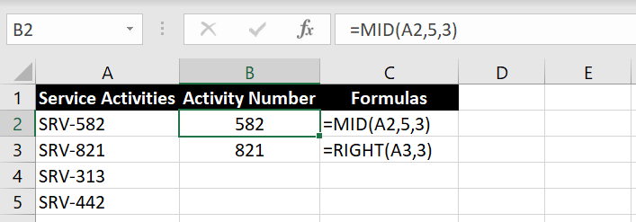
Extract 3 characters in Cell A2, starting with the 5th character
We can see with the example under the MID function, we can get the same result with RIGHT function in this case. But of course this is because our set of data is consistently starting with “SRV-” and ending with a three-digit number. But note that again the number we enter for num_chars could be larger than number of characters available. This could actually be useful, especially if the SRV number is not always 3-digits:

Extracting Substring After a Certain Symbol in a Text
In the previous section, we explored datasets that are relatively uniform and consistent. All the service activities numbers consistently started with “SRV-“. What if we are faced with example below where we would like to extract the surnames out of a list of full names:

This would require more than a simple LEFT, RIGHT or MID functions on their own because the number of characters vary with each name.
So how do we do this? Well we know that the one thing that is consistent between all the names is that the first name and last name are separated by a space in between. So first we need to find the location of the space within the string. Here we will introduce the FIND function.
FIND
The FIND function helps us find a particular character within a text. The function is:
=FIND(find_text, within_text, [start_num])
- Find_text: the character(s) we are looking for
- Within_text: the cell where we are searching for the character(s)
- [Start_num]: from which character should Excel start searching. The square bracket means this is an optional field. By default, it will start searching from the very first character from the left. However we can also get Excel to start searching after nth character.
What FIND function returns is the position or location of the “find_text” character within the “within_text”. Using the example above with the list of full names, we can find the position of the space within each string using the FIND function:

After finding where the position of the space within each string, we can apply it with the MID function. Remember, the MID function allows us to extract text starting from any particular position we nominate.

=MID(A2, “FIND(” “, A2)+1, 50)
- Text: A2 – this is the cell we want the MID function to extract text from
- Start_num: FIND(” “, A2) + 1 – this is the location of the space between first name and last name. But because we don’t want to extract the space as well, we need to add +1 at the end so Excel starts extracting from the first letter of the last name
- Num_chars: 50 – here we specify how many characters we want Excel to return starting from the first character of the surname. Because different surnames would have different numbers of characters, we put 50 hoping no surnames would have more than 50 characters. But the idea is to put in a ridiculously large number so that Excel will capture everything from the first character of the last name to the rest of the string.
Following very similar logic, we can also extract the first names from this list:
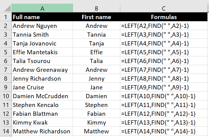
=LEFT(A2, FIND(” “, A2)-1)
Starting from the left, we just need to tell Excel how many characters we want to extract. And again we use the FIND function to find the first space. In this case, we need to add -1 so that the space will not be extracted as well.
A More Complex Example with Middle Names
To complicate the situation a bit more, let’s have a look at the dataset below and we want to extract the middle name. Note that not everyone in the list has a middle name:

In this case, we cannot start from the left or from the right so we need to use the MID function. To use the MID function to extract the middle name, we will need the following:
- The cell to find middle name: A2
- Where to start extracting – in this case, after the first space: =FIND(” “, A2)+1
- The number of characters we want to extract – in this case, it is the number of characters the middle name has. The most simple way to think about this is the position of the second space minus the position of the first space.

Looking at the picture above, 1) is the position of the first character of the middle name, 2) is the position of the second space and finally 3) is the difference between 2) and 1) and it is the number of characters the middle name has.
- Position of the first character of the middle name: =FIND(” “, A2)+1
- Position of the second space – this one is slightly trickier. Remember with the FIND function, we have an optional [start_num] field which we can tell Excel where to start looking for a character. In this case we want Excel to start looking for the space after the first one: =FIND(” “, A2, FIND(” “, A2)+1)
- Putting 1) and 2) together, we get the number of characters the middle name has: =FIND(” “, A2, FIND(” “, A2)+1)-(FIND(” “, A2)+1)
So now we can put everything together into the MID function:
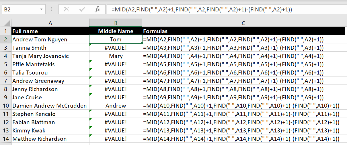
=MID(A2,FIND(” “,A2)+1,FIND(” “,A2,FIND(” “,A2)+1)-(FIND(” “,A2)+1))
Why are some results coming back with #VALUE? The reason is that some people in the list don’t have middle names so after the first space, Excel is not able to find the second space. An easy solution will be to use the IFERROR function:
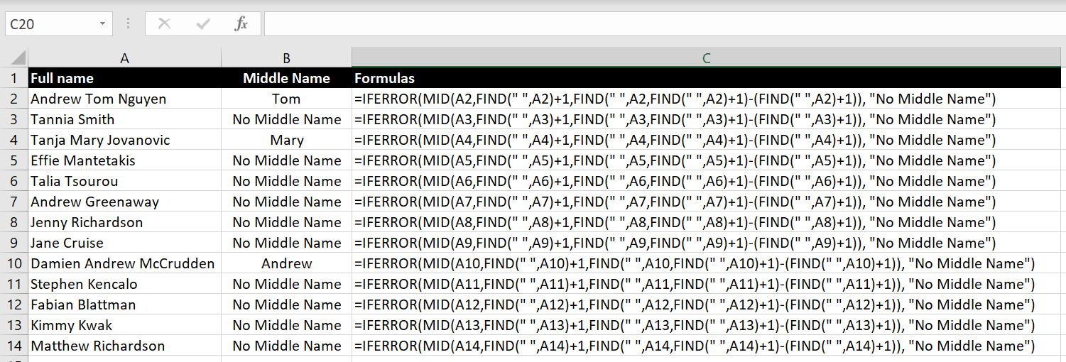
=IFERROR(MID(A12,FIND(” “,A12)+1,FIND(” “,A12,FIND(” “,A12)+1)-(FIND(” “,A12)+1)), “No Middle Name”)
Extracting Last Name When the Full Name has a Middle Name
What if in this case we have a list of full names which have middle names and we want to extract the last names? E.g. below:

In this case we will use the RIGHT function but first we need to figure out how many characters we want to extract. That is, how long and how many characters the last name has:
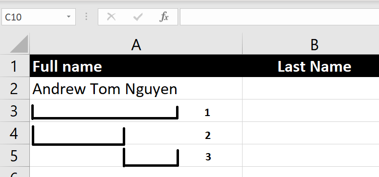
We first need to work out:
- The total length of the string: =LEN(A2)
- The position of the second space in the string: =FIND(” “, A2, FIND(” “, A2)+1)
- The difference between 2) and 1) is the length of the last name: =LEN(A2)-FIND(” “, A2, FIND(” “, A2)+1)
Putting everything together, the formula becomes:

=RIGHT(A2, LEN(A2)-FIND(” “, A2, FIND(” “, A2)+1))
But What If…There Are Multiple Middle Names…
Very often people have more than one middle name. Using the formula above, we will get the following:

So yes, we could potentially use the RIGHT or MID function again on the Column B to extract the last name. That would be one way of doing it. Alternatively let’s look at another method…
- We will find how many spaces there are in the string: to do this, we will first find the number of characters in the original string. And then we will remove the spaces in the original string using the SUBSTITUTE function and find the number of characters in this new string. The difference between the two will be the number of spaces in the text:
=LEN(A2) – LEN(SUBSTITUTE(A2, ” “, “”)) - With that we will use the SUBSTITUTE function replace that last space with a random unique character:
=SUBSTITUTE(A2, ” “, “@”, LEN(A2) – LEN(SUBSTITUTE(A2, ” “, “”))) - We can then use FIND function to find the position of that unique character:
=FIND(“@”, SUBSTITUTE(A2, ” “, “@”, LEN(A2) – LEN(SUBSTITUTE(A2, ” “, “”)))) - Apply the MID function with above to start extracting string from that position:
=MID(A2, FIND(“@”, SUBSTITUTE(A2, ” “, “@”, LEN(A2) – LEN(SUBSTITUTE(A2, ” “, “”)))), 50)
And this is the result:

And this is it for this topic. As you should see by now, each of the functions mentioned is very simple by itself. But put together, they can be used very creatively. Rather than memorizing the order of how these functions are put together, it is more important to understand how these functions can be used together so you can use them together effectively in your situation.
If you would like us to explore any other specific scenarios, feel free to leave a comment below!

0 Comments Leave a comment