
In the VLOOKUP article, we have looked at some limitations with the VLOOKUP function in Excel. For example, we must start from the leftmost column and look up values on the righthand side. Similarly with HLOOKUP, we must start from the top row and look for values downwards. So if you are looking for a more flexible formula in Excel, INDEX and MATCH functions could be your solution. And they are simple to use. First we will go through the INDEX and MATCH functions separately and then we will explore how they can be used together to do a lookup.
Index Function
The purpose of the INDEX Function in Excel is to:
- Look through an array of data and given a specific row number and a column number, it will return a specific value in that array of data
- =INDEX(Array of data, Row Number, Column Number)
Let’s have a look at the example below. Here we are looking into the A1:C14 array of data and specifically, we want the data in Row 5 and Column 3:
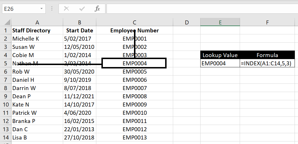
=INDEX(A1:C14, 5, 3)
Match Function
The purpose of the MATCH Function in Excel is to:
- Look through a row/column of data and given a lookup value, it will return where the location of that lookup value is
- =MATCH(lookup value, row/column of data, [match type])
[match type]: similar to VLOOKUP or HLOOKUP, we need to specify whether we want an exact match. 0 is TRUE. 1 is FALSE.
Let’s have a look at the example below. Here we are looking into the array A1:A14 and specifically, we want to know where “Daniel H” is:
- =MATCH(E5, A1:A14,0)
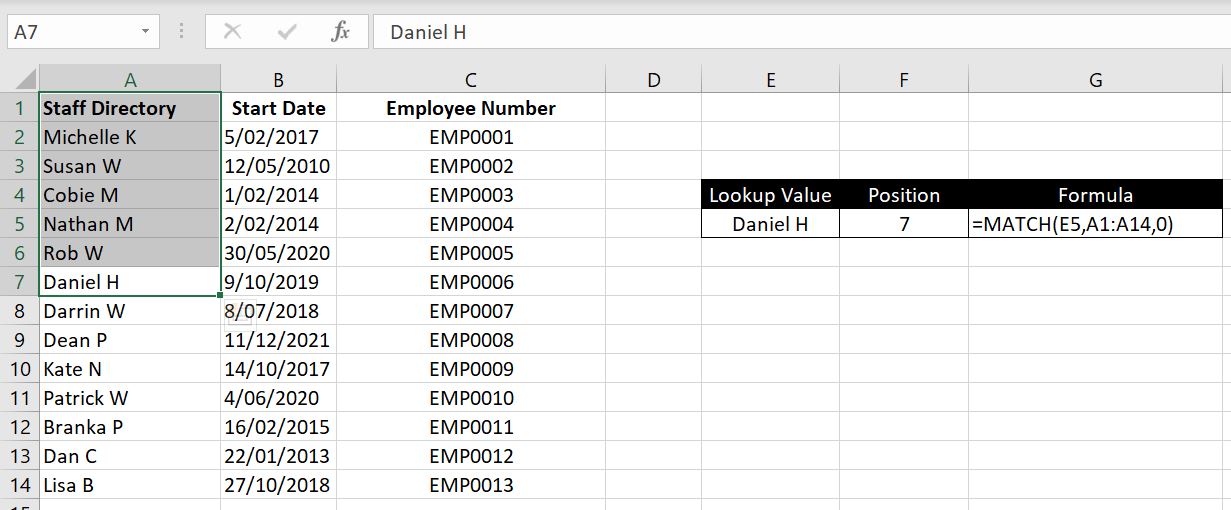
And as we can see, “Daniel H” is in Row 7 and is 7th down the row from A1.
Index Match Functions
Now let’s put the two together. As mentioned above, the INDEX function is:
- =INDEX(Array of data, Row Number, Column Number)
We could now replace the row number or column number (or both) with a MATCH function. Remember, the MATCH function returns the position of a lookup value in a row or column. Once we have the position of the lookup value in a row (or column), we can also specify the column number (or row number) and the INDEX function will return the corresponding value in the array of data.
Example:
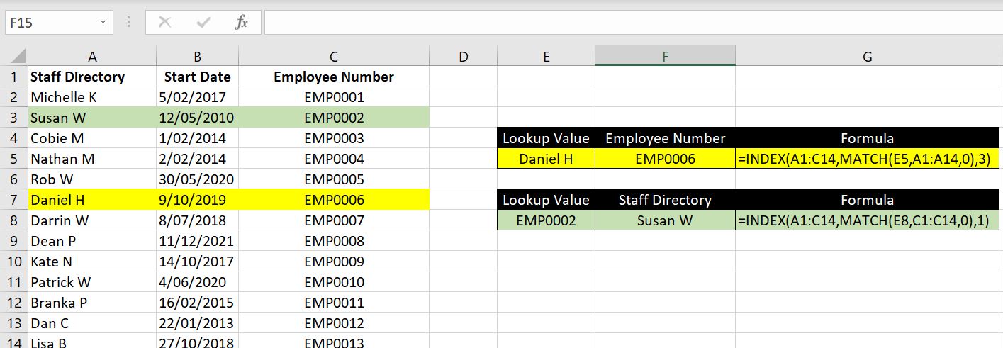
=INDEX(A1:C14, MATCH(E5, A1:A14, 0), 3)
=INDEX(A1:C14, MATCH(E8, C1:C14, 0), 1)
For the first example, we want to find the Employee Number for “Daniel H”. We could easily use the VLOOKUP function (=VLOOKUP(E5, A1:C14, 3, FALSE)). But INDEX and MATCH can work perfectly as well. First we use MATCH function to look up “Daniel H” in A1:A14. This will return 7 as Daniel H is 7th down the list. The INDEX function then becomes =INDEX(A1:C14, 7, 3). 7th row and 3rd column, this will be “EMP0006”.
One thing VLOOKUP will not be able to do though is the second example – working from right to left. In this case, we have “EMP0002” and we want to find who the employee is. First we use the MATCH function to look up “EMP0002” along C1:C14. This will return 3 as EMP0002 is 3rd down the list. The INDEX function then becomes =INDEX(A1:C14, 3, 1). 3rd row and 1st column, this will be “Susan W”.
It works just as well if we replace column number with MATCH function:
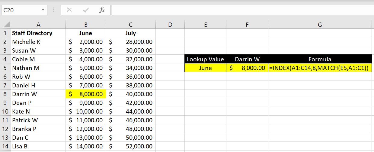
=INDEX(A1:C14, 8, MATCH(E5, A1:C10))
In this case, we want to find “June” amount for Darrin W. Let’s say we already know that Darrin W is in row 8, we then use MATCH function to find “June” across A1:C1 (“=MATCH(E5, A1:C1, 0)). This will return 2 as June is second across the row. The INDEX function becomes =INDEX(A1:C14, 8, 2). 8th row and 2nd column is “$8000”.
Index Match Match Function
Even better, we could replace both row number and column number in the INDEX function with MATCH functions:
Let’s break this down:
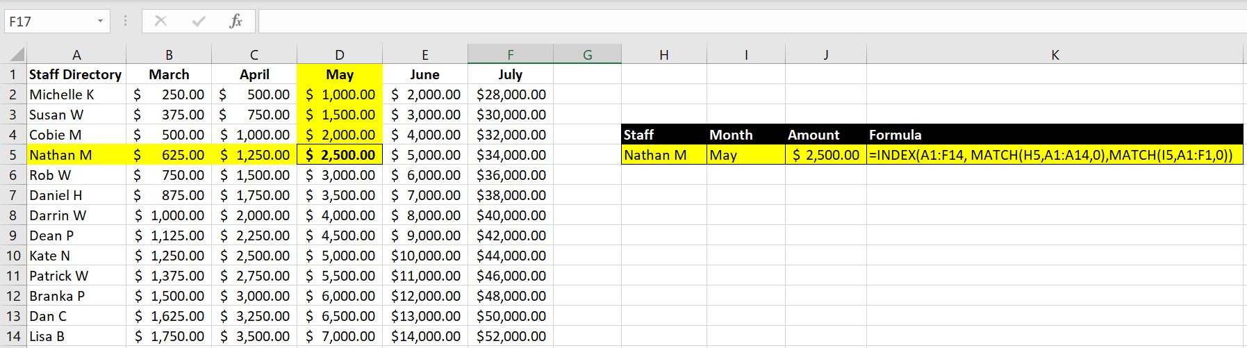
- =INDEX(A1:F14, MATCH(H5,A1:A14,0),MATCH(I5,A1:F1,0))
Row Number – MATCH(H5, A1:A14, 0): this is to search for “Nathan M” along A1:A14. This will return 5 - Column Number – MATCH(I5, A1:F1,0): this will search for “May” along A1:F1. This will return 4.
- Hence the INDEX function is equivalent to =INDEX(A1:F14, 5, 4). Row 5, Column 4 is “$2500”.
Common Errors
We will now look at some of the common errors with Index & Match functions:
- #VALUE: we cannot put in a negative number for row number or column number. This just wouldn’t make sense.
- #REF: when the row number or column number we specified is bigger than the array of data. E.g. with array A1:C5, it would mean there could only be 3 columns. If we specify a column number that is 4 or bigger, INDEX will return #REF.
- Make sure the “array of data” in both INDEX and MATCH function are aligned: this requires more attention because we will not get an Excel error in this case. But the value returned will be incorrect:
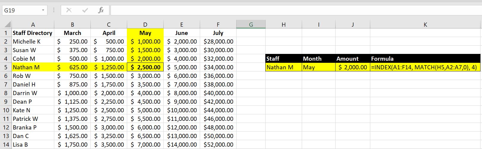
Notice that the returned value is $2000, not $2500. The reason is that the MATCH function is looking at A2:A7 array whereas INDEX function is looking at A1:F14 array. The MATCH function looking for “Nathan M” in A2:A7 means the function will return a value of 4. This means the INDEX function has now become =INDEX(A1:F4, 4, 4). Row 4, Column 4 is $2000.
We hope you now understand how INDEX and MATCH functions work and common errors to look out for. Feel free to leave a comment if we’ve missed anything or if you have any feedback on this article!
0 Comments Leave a comment