Do you want to freeze a row or column in Excel? Do you find yourself constantly having to scroll back up to the top or to the left of the table to look at the headings? For example below, freezing the top row would be very useful because without row 1, we will not know what each number in Column B, C and D refers to.

Freeze Top Row or First Column

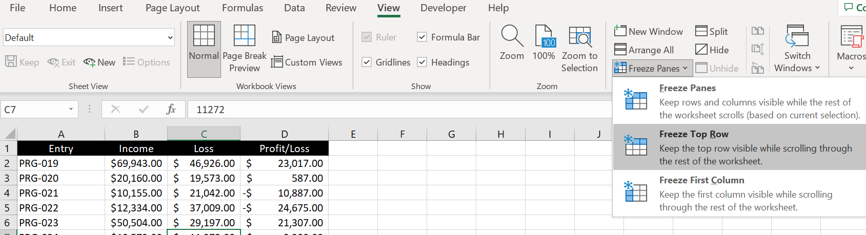
To freeze the top row:

1. Scroll to the top
   
2. Go to View tab
   
3. Click on Freeze Panes
   
4. Select Freeze Top Row
   
   

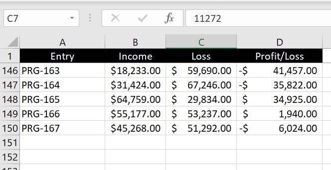
We can now scroll down and Row 1 will always be visible, making it clear what each column is:

And of course we could follow very similar steps to freeze the first column:

1. Scroll to the left
   
2. Go to View tab
   
3. Click on Freeze Panes
   
4. Select Freeze First Column
   
   

And now we can scroll to the right and Column A will always be visible, making it clear what each row is referring to:

Limitation: we cannot use both Freeze Top Row and Freeze First Column together. As soon as you select the other one, the first one disappears. Find out below how we can freeze both row and column.

Freeze Row and Column

There is of course a way to freeze both row and column in Excel. In fact the row and column do not have to be the top row or first column. We could freeze from Row 5 and from Column G if we wanted to. The easiest way would be to:

1. Select the cell which is in the row and column we would like to freeze
   
2. Go to View tab
   
3. Click on Freeze Panes
   
4. Select Freeze Panes
   
   

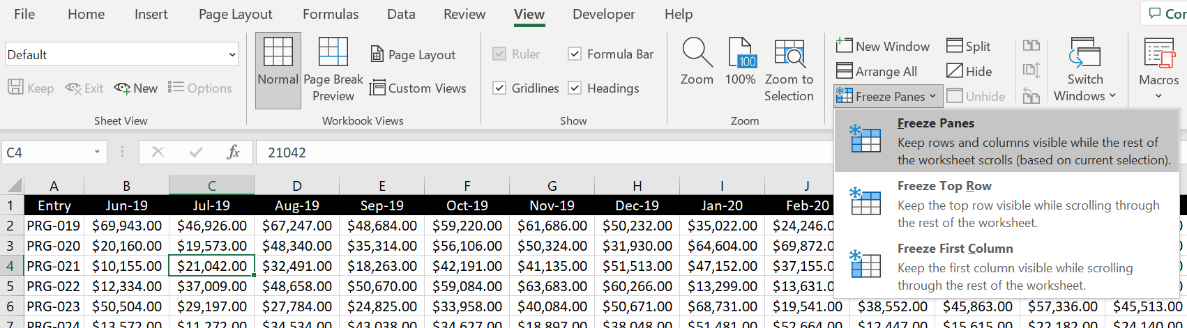
And because C4 was selected in the picture above, Row 3 and Column B will now be frozen:

Freeze Any Row OR Column

In the section above, we went through how to freeze a row and column at the same time. In this section, we will look at how to freeze any row or column and they are not necessarily the top row or first column:

1. Highlight the relevant row or column
2. Go to View tab
3. Click on Freeze Panes
4. Select Freeze Panes
   
   

And as we can see, Column G is now frozen:

Similarly we can do the same thing with any row by first highlighting the relevant row.

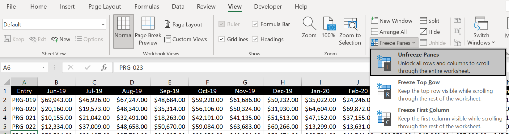
Unfreeze Panes

Unfreezing pane is simple. We don’t even need to highlight the relevant column or row or have the cell selected. We could do so by:

1. Go to View tab
   
2. Click on Freeze Panes
   
3. Select Unfreeze Panes
   
   

Hotkeys for Freezing (or Unfreezing) Panes

To freeze panes using hotkeys:

• ALT > W > F > Choose the following:
  
• F: to freeze or unfreeze pane
  
• R: to freeze top row
  
• W: to freeze first column

And we recommend using the following hotkeys along with freezing panes:

• Shift & space: highlight row
  
• Ctrl & space: highlight column

We hope you find this article useful. If you have any more questions regarding freezing panes in Excel, please leave a comment below and we will keep editing this article to make it more and more useful for everyone.